The Decision Tree Algorithm: Entropy

Which Attribute to Choose? (Part1)

In our last post,  we introduced the idea of the decision trees (DTs) and you understood the big picture. Now it is time to get into some of the details. For example, how does a DT choose the best attribute from the dataset? There must be a way for the DT to compare the worth of each attribute and figure out which attribute can help us get to more pure sub-tables (i.e., more certainty). There is indeed a famous quantitative measure for this called Information Gain. But in order to understand it, we have to first learn about the concept of Entropy. As a reminder here is our training set:

What is Entropy?

Entropy of a set of examples, can tell us how pure that set is! For example, if we have 2 sets of fruits: 1) 5 apples 5 oranges, and 2) 9 apples and 1 orange, we say that set 2 is much more pure (i.e., has much less entropy) than set 1 as it almost purely consists of apples. However, set 1 is a half-half situation and is so impure (i.e., has much more entropy) as neither apples nor oranges can dominate! Now, back to the adults’ world and enough with fruits 🙂 In a binary classification problem, such as the dataset above, we have 2 sets of examples 1) Positive (Yes) and 2) Negative (No), and this is how we compute the entropy of our dataset:
Please note that the base of the Logarithm is 2. As for the proportions, let’s compute them together. We have a total of 11 examples in our dataset with 5 Yes and 6 No. So, the proportions of the class Yes (i.e., positive class) is 5/11 and the proportion of the class No (i.e., the negative class) is 6/11. You notice that the proportions of the positive and negative examples always sum to 1. As a result, we can always say that: P(+) = 1 – P(-). Before showing you a numeric example with decision tree and entropy, I would like to take a moment and analyze the behavior of the Entropy function. Check this out:

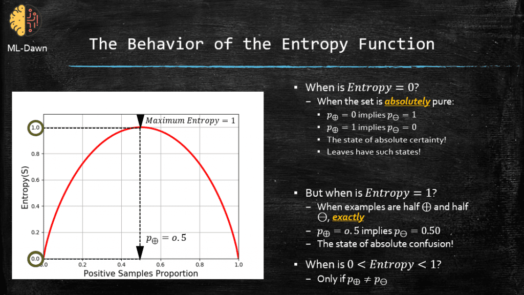
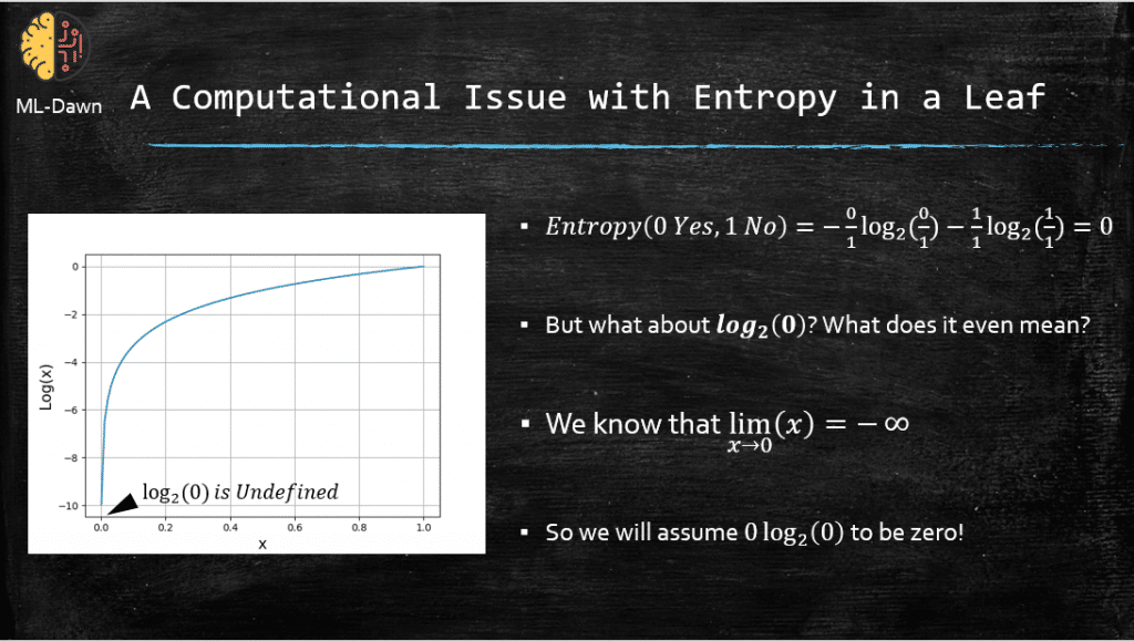
On the horizontal axis we can see the proportion of positive examples (i.e., 1 – Proportion of negative examples) in the set S. On the vertical axis we can see the Entropy of the set S. It seems that this function has indeed a maximum, and it hits 0 ONLY in 2 cases.

In a binary classification problem, when Entropy hits 0 it means we have NO entropy and S is a pure set. So, the members of S are either ALL positive or ALL negative. This is where we have absolute certainty and if you remember in our last post, the leaves of a decision tree are in such state of purity and certainty.

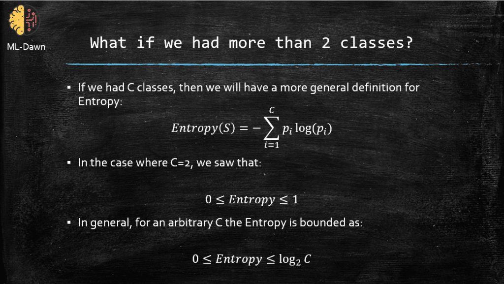
The entropy function for a binary classification has the maximum value of 1. This is the state of utter confusion and highest disorder and entropy. This happens when our set S is EQUALLY divided into positive and negative examples. Meaning that P(+) = 0.5 which automatically implies that P(-) = 0.5.

Finally, in a binary classification problem, if P(+) and P(-) are NOT equal, for example P(+) = 0.7 and P(-) = 0.3, the Entropy is ALWAYS between 0 and 1.

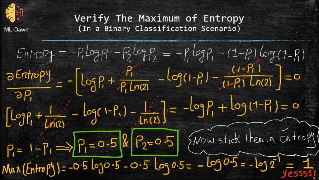
I can actually prove to you that the Entropy for a binary classification problem has a maximum of 1 If and Only If p(+) = P(-) = 0.5. In order to do this, we will have to take the partial derivative of Entropy with respect to one of the proportions (say P(+)), and set it to 0. Then, when we find the critical value for P(+) we can easily find P(-) as we know that: P(+) = 1 – P(-). Finally, by plugging in these critical values for P(+) and P(-) in the Entropy function, we can find the maximum value of the Entropy in the binary classification problem. Below, you can see all the math involved:

This is really cool! Now, we have mathematically proven that ONLY if we have equal proportions between positive and negative example, will the Entropy be maximized and we have determined that maximum value to be exactly 1.

An Illustrative Example

Now, we understand what entropy is as we can apply it to our own training set. Let’s see if we can compute the entropy of our training set. But before we do, what do we expect to get? Should the entropy be close to 1 or close to 0? (hint: compare the 2 proportions)

So this is the starting point where the decision tree (DT) is going to start the training process. Now, in our last post, I showed you how the DT is trained but I never mentioned the concept of Entropy! Now that you know what Entropy is, let’s incorporate that and see whether the DT is trying to increase or decrease the Entropy during the training process. Let’s just focus on the left side of our trained DT and see how the Entropy changes: 

So, even though I still haven’t told you what Information Gain is (except for the fact that it is a way for the DT to choose the best attribute to split the dataset on) we can see that the trend in the Entropy from the starting point of the tree (i.e., the root) all the way to the end (i.e., the leaves) is reduction! So, it seems that training a DT strives to move to the direction of reduction in entropy 🙂

An Issue with Computing Entropy

An observant individual might have noticed that when either of the p(+) or p(-) is 0 we will encounter an interesting situation in computing the entropy! The log(x) when x=0 is not defined! Why? Let’s not forget that Log(x) with the base of a, spits out the power to which you need to raise a to get to x. For example, log(8) with the base of 2 will output 3 and 2 to the power of 3 will give you 8. Now, with this in mind, what do you think of log(0) with the base of 2 (or with any base for that matter!). What real number do you need so if you raise 2 to that real number, you would get 0? There is no such real number! Because we can never get 0 by raising anything to the power of anything. As x gets closer and closer to 0, the log(x) will get smaller and smaller and leans towards -infinity. The real logarithmic function logb(x) is defined only for x>0.So, 0xlog(0) is assumed to be 0 when computing the Entropy! You can see the plot of the log(x) down below and see how steep it reduces around x=0.

What if we had More than 2 Classes?

So far we have been simplifying things and just considered the 2 class case where we have only 2 class labels: Positive and Negative. Let’s get real now! If we have C number of classes, then the formula for the Entropy will look different alittle bit. Moreover, the Entropy can get higher than 1 now! More precisely, the the maximum of Entropy will be log(C)! As a result, if C=4, then maximum Entropy that we could ever observe will be log(4) which is 2! But again the minimum Entropy that we could ever reach to is 0. Check it out:

In the next post, I will tell you how Information Gain uses Entropy to help the Decision tree decide on which attribute to split the dataset on. Spoiler alert: Which attribute will reduce the Entropy the most if we did the splitting on it!

Until then, take care 🙂

MLDawn

Leave a Comment

Your email address will not be published.