The Backpropagation Algorithm-PART(1): MLP and Sigmoid

What is this post about?

The training process of deep Artificial Neural Networks (ANNs) is based on the backpropagation algorithm. Starting with this post, and a few subsequent posts, we will lay the foundation of what a Multilayer Perceptron (MLP) is. We learn how to choose a proper activation function for MLPs and how the backpropagation algorithm works. Below is the video of this whole post if you prefer a video content. Let’s get started 😉  

Deep MLP vs. a Single Perceptron

As we have discussed in our previous post on perceptrons, a perceptron can only learn a linear decision boundary in a classification task, or fit a line to a bunch of data points in a regression task. As a reminder, down below, you can see the architecture of a perceptron with its thresholding step function in its output. 

A perceptron

In contrast to a simple perceptron, a multilayer neural network is capable of learning highly sopisticated decision boundaries for the classification task. It can also fit highly non-linear curves for the regression task. This is the same flexibility that we have with deep learning, mind you! Below you can see the architecture of a deep MLP with a few layers between its input and output layers. 

A quick fact: In order to train a deep neural network, we can use the backpropagation algorithm. The backpropagation algorithm uses the chain rule to backpropagate the gradients throughout the entire network. The gradient descent optimization algorithm then uses these gradients to update the network parameters. Don’t worry, we will dig into these in later posts.

A deep MLP

As you can see, the middle layers no longer deal with the input space. They deal with the outputs of their previous layers to be more precise. In fact, the deeper the data travels through these layers, the more meaningful features are extracted from it.

How to Choose a Threshold Unit?

Each neuron in an ANN has an Activation Function, which we denote with f(). At first this mathematical function, receives the input x (i.e., pre-activation) to the neuron. Next, it does some mathematical manupulation to it (i.e., f()), and finally spits out the result (i.e., f(x)). 

The golden question: How should we choose this f()?

You might be slightly tempted to choose a simple linear function (Discussed in the previous post) for the neurons in your ANN, where for each neuron: f(x) = x.

Congratulations! Now you have multiple layers of cascaded linear units across your entire ANN! The result of many many nested lines is still a line! Thus, your entire ANN still produces linear functions. Under-whelming indeed!

We are interested in ANNs that can represent highly sophisticated non-linear functions, which is the type of problem we face in the real world! So, non-linearity is a desirable feature of an activation function!

Can we use a perceptron unit as our activation function across our ANN? The problem is that the perceptron unit is discontinuous at 0, and hence, non-differentiable at 0. As a result, this makes it unsuitable for gradient descent.\

In conclusion, our expectations from f() are two-fold:

  1. We want f() to be non-linear. This makes the entire ANN a collection of nested non-linear functions, capable of representing some scary non-linear function.
  2. We want f() to be continuous, and differentiable with respect to its input. This makes the entire ANN trainable using gradient descent. Great stuff!

Sigmoid Threshold Unit

The sigmoid function is a function that satisfies both of our requirements, that is, both non-linearity and differentiablity. A sigmoid threshold unit, is actually really similar to a perceptron, but the difference is that it is based on a smoothed and differentiable function, as opposed to the step function that is used in a perceptron. Below, is a visual representation of a sigmoid unit:

a sigmoid unit

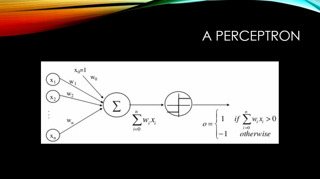
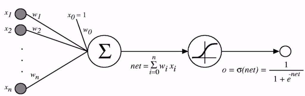
The total input to the sigmoid unit is denoted with net. Very similar to a perfceptron, a sigmoid unit computes a linear combination of its inputs (i.e., net =\sum_{i=0}^{n} w_i \times x_i) and then applies a threshold to the result. However, this threshold output is a continuous function of its input. Mathematically speaking, the sigmoid unit computes its output o as follows:


o = \sigma(\vec{w}.\vec{x})

where

\sigma(\vec{w}.\vec{x}) = \frac{1}{1 + e^{-\vec{w}.\vec{x}}}

\sigma 
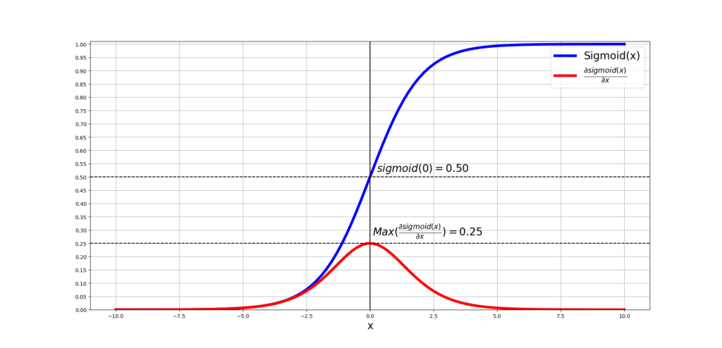
is called the sigmoid function, also known as the logistic function, and this is what it looks like:

sigmoid visualisation

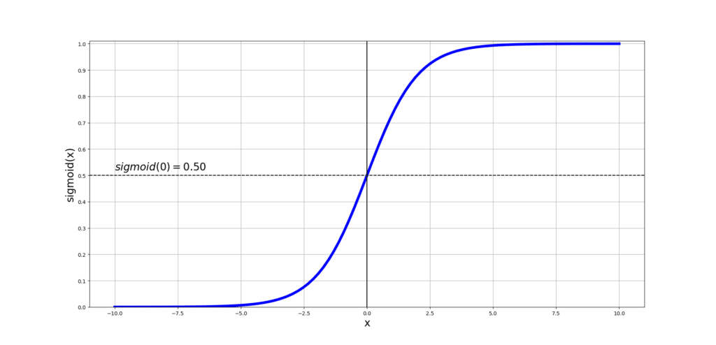
As you can see, the output of sigmoid ranges between 0 and 1, and it increases monotonically with respect to its input.

Fun fact: Since sigmoid can map a large input domain into a small range of  [0,1], it is commonly referred to as the squashing function.

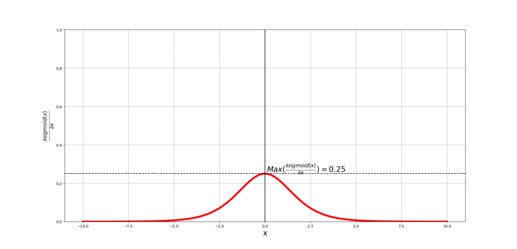
The derivative the sigmoid function with respect to its input can be computed using its output (Dissected in my video: What is the Derivative of the Sigmoid function?):


\frac{d \sigma{(net)}}{dy} = \sigma(net) \times (1- \sigma(net))


which will come in handy when we will talk about the backpropagation algorithm in the next post.

Note: The sigmoid function has certain issues, namely, vanishing gradient and saturation! And that is why people tend to use other activation functions such as the Rectified Linear Unit (Relu). I have dissected Relu and how it solves these issues in an exciting post: Dissecting Relu: A desceptively simple activation function .

Visualising Sigmoid and its Derivative

Let’s first visualize the sigmoid function and then talk about some of its properties. We use Python and Matplotlib to do this.

# Importing the packages
import matplotlib.pyplot as plt
import numpy as np 

Now, we will define 2 functions for computing the sigmoid and its derivative.

def sigmoid(x):
    return 1 / (1 + np.exp(-x))

def derivative_sigmoid(x):
    return sigmoid(x)*(1- sigmoid(x)) 

Define a range of input values for computing the sigmoid and the derivative of sigmoid.

# Input range for sigmoid/derivative_sigmoid
x = np.linspace(-10, 10, 100)
# This will be used for the visualisations later on
font_size = 20 

Let’s plot sigmoid:

plt.figure(figsize=(16,9))
plt.plot(x, sigmoid(x), linewidth=5, c='b')

plt.yticks(np.arange(0, 1.1, 0.1))
plt.xlabel("x",fontsize=font_size)
plt.ylabel("sigmoid(x)",fontsize=font_size)
plt.ylim(0,1.01)

plt.axvline(x=0, c='k')
plt.axhline(y=sigmoid(0), c='k',linestyle='--')
plt.annotate(r'$sigmoid(0)=%.2f$' % sigmoid(0), (-10, 0.52),fontsize=font_size)

plt.grid()
plt.show() 

You can see how the input range that is between [-10,10] is squashed between [0,1]. You also note that the mid-point of sigmoid is where its input is exactly 0, and the output at 0 is exactly 0.5.

sigmoid visualisation

Let’s now plot the derivative of sigmoid over the same range of input values:

plt.figure(figsize=(16,9))
plt.plot(x, derivative_sigmoid(x), linewidth=5, c='r')

plt.xlabel("x",fontsize=font_size)
plt.ylabel(r'$\frac{\partial sigmoid(x)}{\partial x}$',fontsize=font_size)
plt.ylim(0,1)

plt.axvline(x=0, c='k')
plt.axhline(y=derivative_sigmoid(0), c='k',linestyle='--')
plt.annotate(r'$Max(\frac{\partial sigmoid(x)}{\partial x})=%.2f$' % derivative_sigmoid(0), (0.1, 0.26), fontsize=font_size)

plt.grid()
plt.show() 

You can see that the derivative is always positive and approaches 0 on the two extremes. The maximum value of the derivative again happens at x=0 and it is 0.25.

sigmoid derivative visualisation

Now, let’s plot both plots in one figure and see the overlaps and understand what they mean:

plt.figure(figsize=(16,9))
plt.plot(x, sigmoid(x), linewidth=5, c='b', label='Sigmoid(x)')
plt.legend(fontsize=font_size)
plt.axvline(x=0, c='k')
plt.axhline(y=sigmoid(0), c='k',linestyle='--')
plt.annotate(r'$sigmoid(0)=%.2f$' % sigmoid(0), (0.26, 0.52),fontsize=font_size)

plt.plot(x, derivative_sigmoid(x), linewidth=5, c='r', label=r'$\frac{\partial sigmoid(x)}{\partial x}$')
plt.legend(fontsize=font_size)
plt.axhline(y=derivative_sigmoid(0), c='k',linestyle='--')
plt.annotate(r'$Max(\frac{\partial sigmoid(x)}{\partial x})=%.2f$' % derivative_sigmoid(0), (0.1, 0.28), fontsize=font_size)
plt.xlabel("x",fontsize=font_size)
plt.yticks(np.arange(0, 1.1, 0.05))
plt.ylim(0,1.01)

plt.grid()
plt.show() 

What can we understand from this? So this means that if the input of the sigmoid is really large or really small, the derivative of sigmoid with respect to those particular extreme inputs appraoches 0. At 0, we can already see that the derivative is at its peak and this makes sense since the slope of the tangent line on sigmoid at 0 is the steepest.

sigmoid and its derivative

Conclusions

Adding more layers to a neural network and creating a multilayer network, with non-linear activation functions in these neurons can make our Artificial Neural Network (ANN) really flexible and capable of learning more sophisticated patterns in the input data. We have also seen that the activation functions used in these networks need certain properties: 1) Differentiability 2) Non-linearity and we have studied the sigmoid function as a candidate of such functions.

In the next post we will start our discussion on the backpropagation algorithm.

Until then,

On behalf of MLDawn,

Take care 😉

Leave a Comment

Your email address will not be published.