What will you learn?
You will learn how a decision tree works but without going to the details. For example, you will NOT learn about Entropy and Information Gain in this post. However, you will have a broad and nice understanding about how a decision tree works. I do hope that you will find it useful and worth your while. Enjoy 🙂
Decision Trees: Introduction
A decision tree (DT) is nothing but yet another algorithm that helps us make classifications on a bunch of data. It is a machine learning algorithm so we will need some training data, which will have some attributes, and this is where the DT comes into play! Is takes a look at your table of training data, and also the ground truth labels! Then it will choose an attribute from the table, and using its values across the whole training set, it will split the whole table into 2 halves! And then in each sub-tree it will do the same until we reach the leaves that correspond to the ground truth! The criterion for stopping the split is a concept called the purity of the current set at hand. If it is confusing, no worries, here is an illustrative example. Watch carefully! This is the training data that the DT will slice up soon 🙂
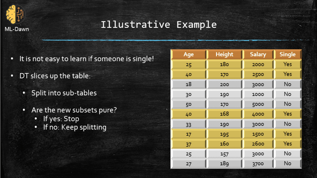
So we have 3 attributes: Age, Height, and Salary
And the concept that we are trying to learn and, hopefully, predict is called “Single”. So if we know the values of these attributes for a person, can we determine whether they are are single or in a relationship! Perfect! Here is the first question before anything starts: How pure is this set of data?
Well currently we have a mixture of labels in the set: 5 Yes and 6 No! So, it is not pure at all, in fact it is nearly a mix of the 2 labels. You see where I am going with this right? We want to break this bloody table in a way that we will end up with a pure set, so we will have either ALL yes’s or ALL No’s and that is what we call a pure set, and that’s it!
Now, the DT chooses an attribute (Don’t ask how, I will elaborate in the next post :-)), and slices the whole training data into 2 halves, and then does that again, and again, until we reach to a determined answer for the target value (i.e., the concept we want to learn) which is the concept of “Single”. Here are the steps:
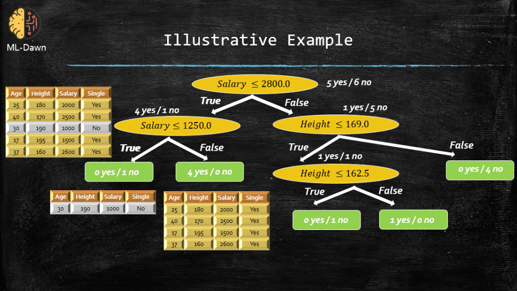
So, the DT chose the attribute Salary and then chooses a splitting value 2800.0, then splits the whole table! All the rows for which the condition Salary <= 2800.0 holds will be sliced and put in the left side of the tree (I have put this sliced up table on the left side for you). All other rows for which the condition doesn’t hold will be sliced and set to the right side of the tree. Now, let’s focus on the left side: Look at the table, is it a pure set? Well we have 4 Yes’s and 1 No! So, it is not yet pure and we need more splitting. DT again chooses “Salary” but this time splits this table using a different threshold: 1250.0. As you can see the resulting tables are both pure now. One has 0 Yes and 1 No, while the other has 4 Yes’s and 0 No! So we will no longer have to split these! So, you get the idea, and I am sure you can follow the right hand side of this whole tree 😉
Now, the training is done and we have constructed our trained DT. Let’s see what sorts of rules has the DT learned to explain the concept of “Single”:
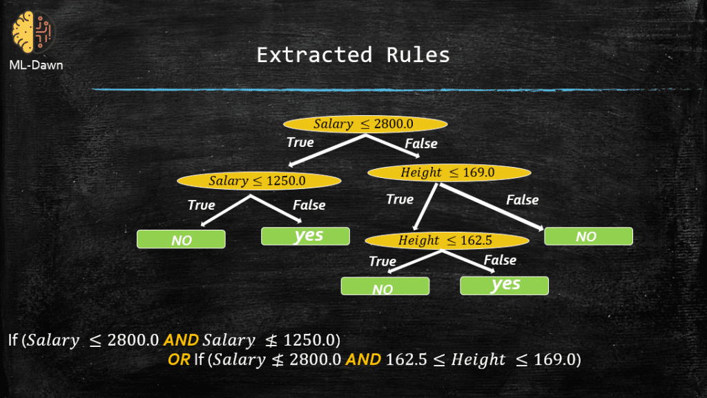
So, this means that the DT thinks, given the attributes we have seen, there are mainly 2 ways to determine whether a given person is single: 1) Their Salary is below 2800.0 but higher than 1250 OR 2) Their Salary is higher than 2800.0, and their Height is between 162.5 and 169.0.
Obviously, this is just an example and these rules simply mean nothing in real life. Have fun with the example and learn the concept 🙂
Now, I am intrigued to test this tree. Imagine if this new person that we have not seen before, and we ask their Age, Height, and Salary (A little rude to do this last bit but it is just an example :-)), and we want to predict whether they are single or not and we will consult our tree to figure this out.
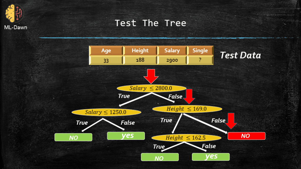
So, they are 33 years old, and quite tall 188, with the salary of 2900.0! Now, the DT checks the salary which is NOT less than 2800.0 so we go to the right side of the tree. Next it check the Height, which is NOT less than 169.0 so we reach to the Leaf of the tree which says: No! So, we believe that this person is in a relationship and that’s it!
Implementation in Scikitlearn & Python
PLEASE NOTE: These codes are snapshots just to encourage you to type the commands yourselves. Believe me when I tell you that, as painful as this might seem, it is the only way to learn the coding bit 😉
Now back to business, let’s see how we can implement this very problem in Python. Please note that this is not coding from scratch and I am using Scikitlearn. Below you can see the training phase in all its glory. The code is well commented so I do hope that it is clear:
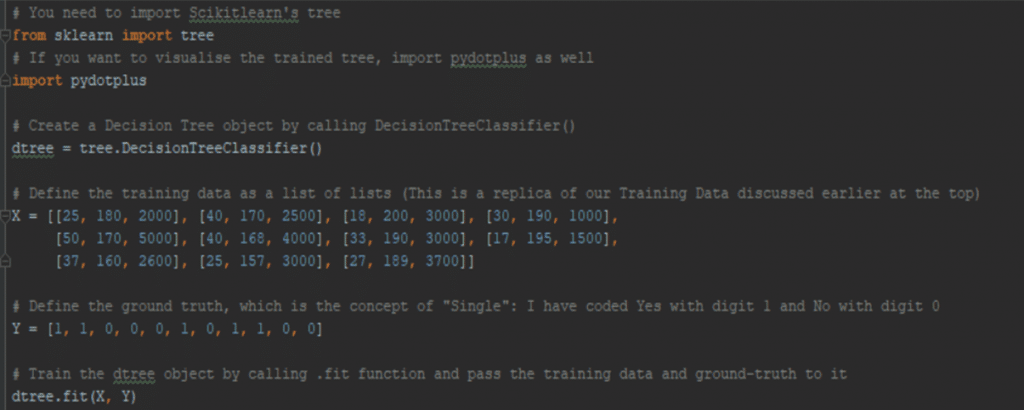
At this stage the dtree object is a trained Decision Tree (DT). I am sure that you want to visualise it as well! After all a tree should look cooler than a script, right?

Now you should have a file named dtree.png in the same directory that you are running this code. If you open it, you should see a visualisation identical to the one below:
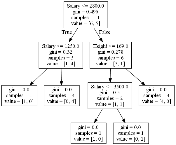
This is basically the exact same visualisation that I showed you at the top of this page. Now, you might find certain things confusing in this .png file though! What is the world is gini? This is actually a well-defined mathematical metric that can tell you how pure your current set is! I will elaborate on this in the next post. The variable Samples at each node, tells you about the number of entries in the table that has survived the conditions up to that particular node. Basically, this is the sum of the entries (i.e., all Yes’s and No’s)! Moreover, value [6, 5] in a node means that we have 6 entries with ground truth label No and 5 entries with ground truth label Yes. If you notice the leaves, you can see that we have at least one 0 in the variable value! This means that all leaves are pure! Meaning that either ALL the entries in them are Yes’s or ALL of them are No’s. That is why they are the leaves and that is why we have stopped splitting further 🙂
Now it is time to show you how you can test this tree in Python. We define our test data and then simply call the .predict() function in the our DT object dtree. Please note that we are testing the tree with the same test data I showed you earlier in this post, so we have to expect identical result, which is in this case: No meaning that the DT has to predict that this new person is NOT single.

And sure enough, this will output a 0 for us referring to the class No. This is what we have confirmed by hand in this post.
What is Next?
In the next post, I will tell you more about how the DT chooses the attribute on which to do the splitting. This is by no means random, as I am sure you know by now. In particular we will talk about: Entropy and Information Gain
