Back-propagation with Cross-Entropy and Softmax

Home

/

Back-propagation with Cross-Entropy and Softmax

What will you learn?

This post is also available to you in this video, should you be interested 😉

In our previous post, we talked about the derivative of the softmax function with respect to its input. We indeed beautifully dissect ed the math and got comfortable with it! In this post, we will go one step further! Let’s say you have a neural network with softmax output layer, and you are using the cross-entropy error function. Today, we will derive the gradient of the cross-entropy error with respect to the input of the softmax function.

This is one of the most confusing mathematical derivations that machine learning enthusiasts tend to have problems with. This post is important as it shows you, if you have a softmax output layer, and use the cross-entropy function, how you can apply back-propagation from the error all the way to the input of the softmax layer, which is the tricky part of the entire back-propagation in this type of neural networks.

A Typical Neural Network

Let’s consider a simple neural network with D-dimensional input data, and $H$ output neurons with softmax output function. So, for $H$ output neurons, we will have $H$ softmax outputs. We will have one-hot encoding ground-truth vectors and finally we will have the cross-entropy error function to compute the distance between the output vector and the ground-truth vector. This is a typical neural network for a multi-class classification task. So, for a given training example as the input, the network will generate an output vector with the size of $H$ (which is the number of classes in our dataset)!

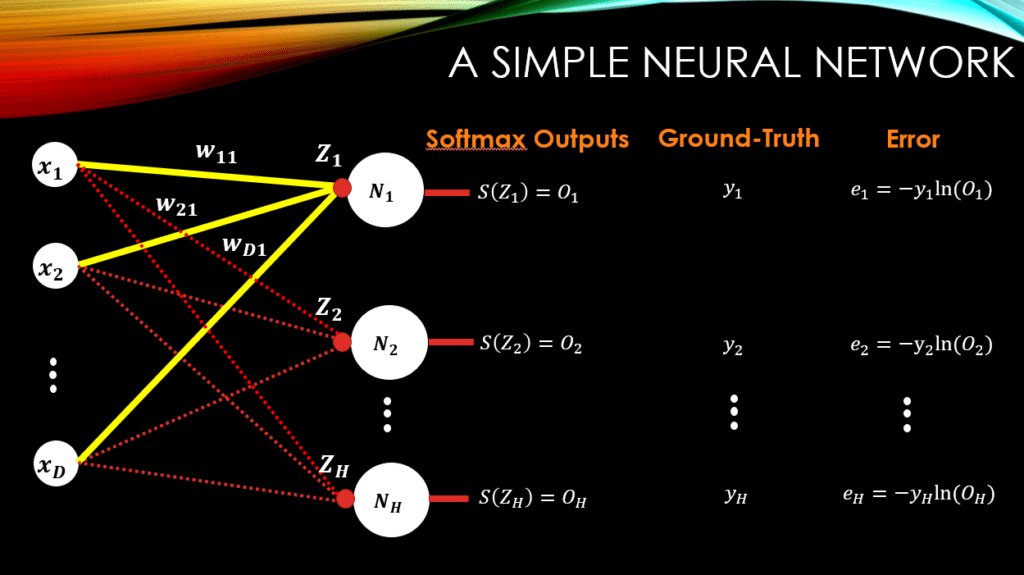
So, just as a gentle reminder, the softmax function can be defined as:

$S(Z_k)=\frac{e^{Z_k}}{\sum_{i=1}^{H} e^{Z_i}}$

And the interesting property of this function is that the sum of all the outputs of softmax, is always equal to 1:

$\sum_{i=1}^{H}S(Z_i)}=1$

Now, about the ground-truth vector, $y$ , we mentioned that it is a one-hot encoding vector. This means that for every ground-truth vector ONLY one element can be equal to 1 and all the other elements are equal to 0!

Finally, regarding the cross-entropy error function, the mathematical representation of this function is as follows:

$E(y, S(Z)) = -\sum_{i=1}^{H}y_i \times ln(S(Z_i))$

In this definition of error, $ln$ , is the natural logarithm. As for an example, let’s say we have 3 output neurons. For a given training example, the output vector of this neural network will have 3 elements in it. Let’s say the output vector is as follows:

$S(Z)=[S(Z_1), S(Z_2), S(Z_3))] = [0.2, 0.6, 0.2]$

You notice that these sum up to 1 as the property of softmax function. And, let’s say the ground-truth vector for the same input training example is as follows:

$y=[y_1, y_2, y_3] = [1,0,0]$

With s simple comparison between the network output vector and the ground-truth vector you can see that, the network thinks that the given training example belongs to class 2 (as 0.6 is the largest value and corresponds to class 2), however, the ground-truth says that the training example actually belongs to class 1 (as only the value corresponding to the first class is 1 and all the others are 0).

Now, let’s see how we can compute the cross-entropy error function:

$E(y, S(Z)) = -(y_1\times ln(S(Z_1))+y_2\times ln(S(Z_2))+y_3\times ln(S(Z_3)))$

which is equal to:

$E(y, S(Z)) = -(1 \times ln(0.2) + 0\times ln(0.6) + 0 \times ln(0.2))=-ln(0.2)$

which is:

$E(y, S(Z)) = 1.6094$

Now that we are comfortable with the whole setting, let’s see how we can derive the gradient of this error function with respect to the inputs of the softmax output function and apply back-propagation from scratch!

Deriving Back-propagation through Cross-Entropy and Softmax

In order to fully understand the back-propagation in here, we need to understand a few mathematical rules regarding partial derivatives.

Rule 1) Derivative of a SUM is equal to the SUM of derivatives

Rule 2) The rule of Independence

$\frac{\partial [f(x)+ g(x)]}{\partial x} = \frac{\partial f(x)}{\partial x}+\frac{\partial g(x)}{\partial x}$

$\frac{\partial [f(x) \times g(y)]}{\partial x} = g(y) \times \frac{\partial f(x)}{\partial x}$

Rule 3) The Chain Rule

if $u$ is a function of $x$ (i.e., $u(x)$ ) and $f$ is a function of $u$ (i.e., $f(u)$ ) then:

$\frac{\partial f}{\partial x} = \frac{\partial f}{\partial u} \times \frac{\partial u}{\partial x}$

Rule 4) Derivative of the log function

$\frac{\partial log_b (x)}{\partial x} = \frac{1}{ln(b) \times x}$

You can see that we could easily extend Rule #4 to the natural logarithm where the base of the logarithm is the Euler’s number (i.e., 2.7182 …):

$\frac{\partial ln (x)}{\partial x} = \frac{1}{ln(e) \times x} = \frac{1}{x}$

This happens because $ln(e) = 1$ .

In order to derive the back-propagation math, we will first have to compute the total error across all the output neurons of our neural network and only then can we start with our derivatives and back-propagation. So, we will sum up all the individual errors, $e_i$ , for $i\in \{1,2,...,H}\$ , and this will be total error across all output units!

NOTE: In this example, this total error corresponds to the output of the network for ONLY one input training example! Meaning that, if we wanted to compute the error across the whole training examples, we should add another summation to our error computation: $\sum_{d \in D} \sum_{i=1}^{H} e_{di}$ where D is the entire training set. In here, $e_{di}$ corresponds to the error value in the $i^{th}$ output neuron when the $d^{th}$ training example is fed to the neural network.

Now, in order to apply back-propagation, we will have to compute the gradients of the total error w.r.t the inputs of the softmax layer. Please note that this is only the beginning of the back-propagation! If you had 20 layers in your neural network, you would have to compute the gradient of your error w.r.t all the learnable parameters across all 20 layers! However, I believe this initial part is the step where most people are not quite comfortable with. Now, let’s see how we can compute the gradient of the total error w.r.t the inputs of the softmax layer:

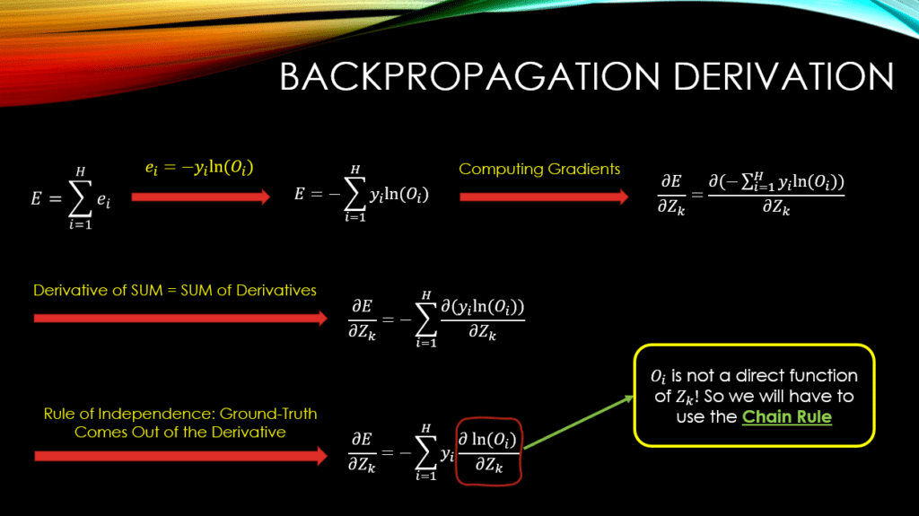
You can see that we have subtly used Rule #1, in order to take the partial derivative operation into our SUM! And we have also grabbed our ground-truth variable $y_i$ out of the partial derivative operation, using Rule #2 of independence! Because our ground-truth variable is independent of all the inputs to our softmax layer, $Z_k$ ! As a result, we can treat it as an independent variable from

$Z_k$ , and bring it out of the partial derivative operation! Finally you notice that we will have to use Rule #3, that is the chain rule!

Why the chain rule? Well because in $\frac{\partial ln(O_i)}{\partial Z_k}$ , we notice that $ln(O_i)}$ is not a direct function of $Z_k$ ! However, it is a direct function of $O_i$ ! In turn, $O_i$ is indeed a direct function of $Z_k$ ! So, in order to compute $\frac{\partial ln(O_i)}{\partial Z_k}$ , we will have to go through $O_i$ first and then get to $Z_k$ ! By chaining these steps together we will have our chain!!!

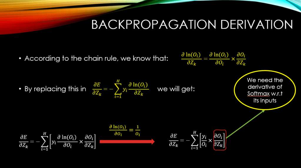
Now after applying the chain rule, you notice that we have also used Rule #4 to find the derivative of our natural logarithm, that is, $\frac{\partial ln(O_i)}{\partial O_i}$ . We have got to the place where we will need the derivative of the softmax function w.r.t its input (i.e., $\frac{\partial O_i}{\partial Z_k}$ ). We have already covered the derivative of softmax w.r.t its input in our previous post, but as a reminder, see the slide blow:

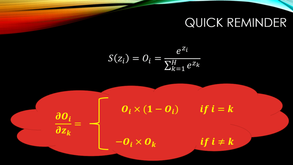
So, we can see that when it comes to $\frac{\partial O_i}{\partial Z_k}$ , it all boils down to whether $i=k$ or $i \neq k$ ! As a result, in order to compute $\frac{\partial O_i}{\partial Z_k}$ , for a given $Z_k$ , we will consider all $O_i$ ‘s for $i \in \{1,2,...,H}\$ ! There will be ONLY one case where $i=k$ , and for all other values of $i$ , for sure we will have $i \neq k$ ! Thus let’s solve $\frac{\partial O_i}{\partial Z_k}$ for both cases:

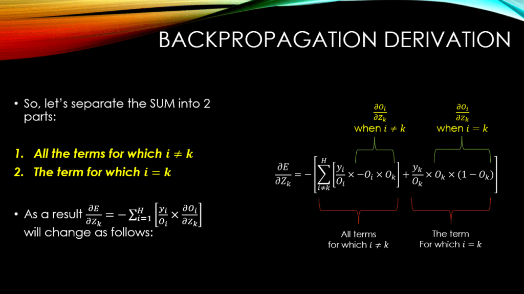
Now, the hard part is over! You can see how we have taken out the term for which $i=k$ ! Then we have used the derivative of softmax (extensively discussed in our previous post) in order to finally be done with the partial derivative operations. Now, let’s simplify:

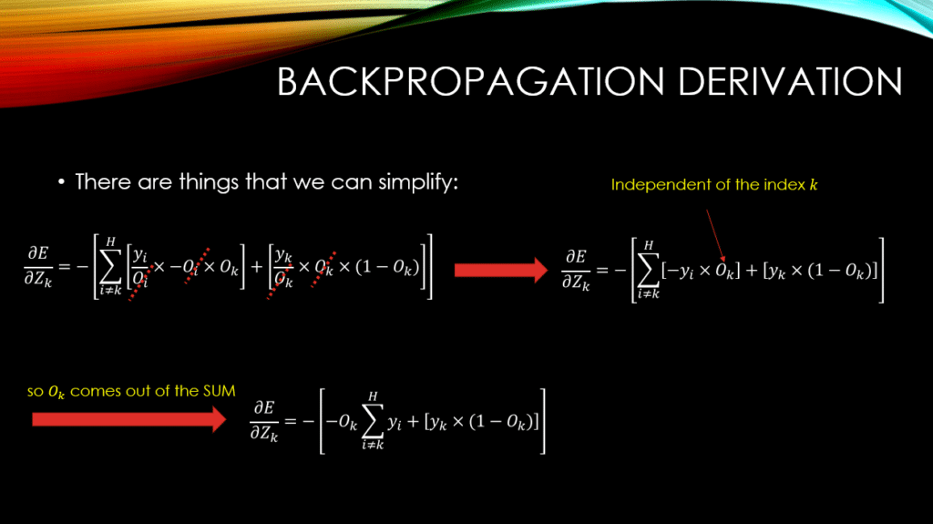
You notice that $O_k$ has come out of the SUM! The reason is simply because, the index of $O_k$ , is independent of $i$ , that is the index over which we are summing! So, $O_k$ is treated as a constant coefficient of $y_i$ !

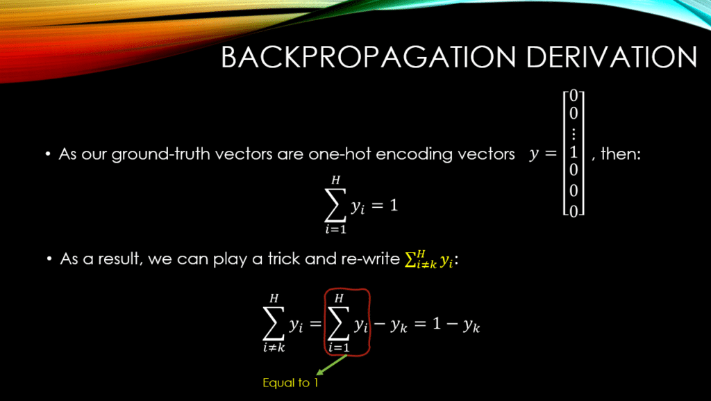
In order to get rid of the summing operation, the next trick we can play is taking advantage of the fact that, the ground-truth vector $y$ , is a one-hot encoding vector! As a result, if we sum all of its elements across all $H$ outputs, the result will always be equal to 1 (i.e., $\sum _{i=1}^{H} y_i =1$ ). So, in order to compute $\sum _{i \neq k}^{H} y_i$ , we can subtract the $k^{th}$ element of $y$ (i.e., $y_k$ ), from $\sum _{i=1}^{H} y_i$ . This is how we will get rid of the SUM from our math! See below:

So, now that we have computed $\sum _{i \neq k}^{H} y_i$ with our smart approach, let’s replace it in our derivations, and simplify more:

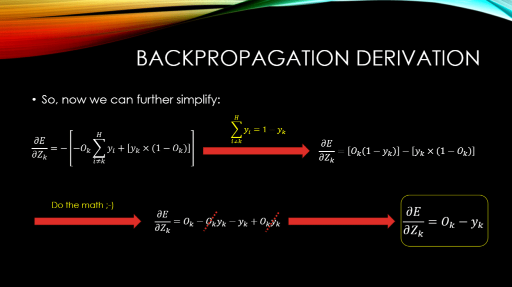
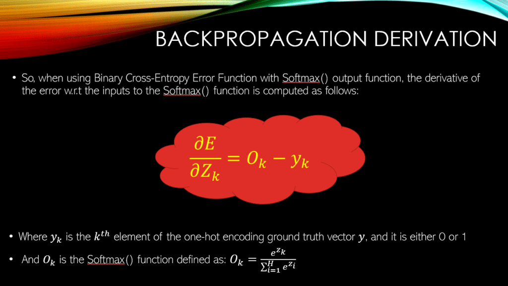
Perfect! We are finally done! Let’s see the final answer in a nice and concise way:

Conclusions

So there you have it! Now you can see the very simple outcome of this whole monstrous series of derivations! The fact that it could be simplified to this level, is the benefit of using the cross-entropy error function with softmax output function in neural networks! However, this simplicity is not the main reason as to why we use softmax coupled with cross-entropy error function, mind you! This is just the nice outcome that we can enjoy!

Until next time, on behalf of MLDawn

Take care 😉

Author: Mehran

Dr. Mehran H. Bazargani is a researcher and educator specialising in machine learning and computational neuroscience. He earned his Ph.D. from University College Dublin, where his research centered on semi-supervised anomaly detection through the application of One-Class Radial Basis Function (RBF) Networks. His academic foundation was laid with a Bachelor of Science degree in Information Technology, followed by a Master of Science in Computer Engineering from Eastern Mediterranean University, where he focused on molecular communication facilitated by relay nodes in nano wireless sensor networks. Dr. Bazargani’s research interests are situated at the intersection of artificial intelligence and neuroscience, with an emphasis on developing brain-inspired artificial neural networks grounded in the Free Energy Principle. His work aims to model human cognition, including perception, decision-making, and planning, by integrating advanced concepts such as predictive coding and active inference. As a NeuroInsight Marie Skłodowska-Curie Fellow, Dr. Bazargani is currently investigating the mechanisms underlying hallucinations, conceptualising them as instances of false inference about the environment. His research seeks to address this phenomenon in neuropsychiatric disorders by employing brain-inspired AI models, notably predictive coding (PC) networks, to simulate hallucinatory experiences in human perception.

Add a comment

By using form u agree with the message sorage, you can contact us directly now

Responses

Moin November 24, 2021

Great tutorial and explanation! Only thing i would fix are the images (equations) showing the rules of partial derivatives. They are overlapping the text

Reply
1. Mehran November 24, 2021
  
  Thanks for the feedback. Duely noted!
  
  Reply
Ali January 31, 2022

Great explanation!

Reply
1. Mehran April 2, 2023
  
  I am glad it was helpful 🙂
  
  Reply
Oliver March 21, 2022

This is by far the best explanation on the internet. I’ve spent like 3 hours looking for answers and every website or video I’ve come by has repeatedly done incomprehensible shortcuts that convolute the process so much. This was a very by the textbook, simple derivation. Longer but way more understandable.

Reply
1. Mehran April 2, 2023
  
  My suffering was identical to your when I was learning about this topic! This was the main reason why I created this tutorial!
  
  Reply
Jano April 1, 2022

Hi, thanks for the explanation, really clear and easy to follow. However, I don’t understand why we are calculating the derivative of the loss w.r.t. the softmax, instead of calculating the derivative of the loss w.r.t. the weights.

Reply
1. Mehran April 2, 2023
  
  Here is the catch! The only way you can compute the derivative of lthe loss w.r.t the weights, is to go through the softmax function (according to the Chainrule).
  
  Reply
  1. Tanjim November 11, 2023
    
    what will be the equations for updating weights in an input-hidden layer?
    Could you please write it down.
    
    Reply
  2. Albir November 11, 2023
    
    what will be the laws of updating hidden and input layer weights!
    
    Reply
fishfin November 3, 2022

I am doing a DataScience course, and apart from the uses of Softmax in classification problems, no-one talks anything more about it. Having understood back propagation to a reasonable extent on YT and such, I was very curious on how it works with Softmax, and this article explained it pretty clearly. Apart from Softmax, I am also interested in understanding the mechanics of MaxPool, Dropout, BatchNormalization, specifically wrt back propagation, any pointers?

Reply
1. Mehran April 2, 2023
  
  Cool! Please be more specific about your questions 🙂
  
  Reply
Shounak January 13, 2023

Finally, I found a good explanation for this topic. Other articles were way too difficult for a beginner like me to understand. Splendid JOB !!

Reply
1. Mehran April 2, 2023
  
  Perfect 🙂
  
  Reply
qaz July 11, 2023

this is by far the best explanation of backpropagationw with CE and softmax that i’ve seen, but i still got a question that are the derivatives of E with resoect to every Z same? because O-k and Y-k are fixed values in every sample, right?

Reply
qaz July 11, 2023

This is by far the best explanation of backpropagation with cross-entropy and softmax that I’ve seen. However, I still have a question: are the derivatives of E with respect to every Z the same? This is because O-k and Y-k are fixed values in every sample, right?”

Reply
qaz July 11, 2023

This is by far the best explanation of backpropagation with cross-entropy and softmax that I’ve seen. However, I still have a question: are the derivatives of E with respect to every Z the same? This is because O-k and Y-k are fixed values in every sample, right?”

Reply
qaz July 11, 2023

This is by far the best explanation of backpropagation with cross-entropy and softmax that I’ve seen. However, I still have a question: are the derivatives of E with respect to every Z the same? This is because O-k and Y-k are fixed values in every sample, right?”

Reply
Anonymous November 11, 2023

what will be the equation of chain rule? When we want to update input-hidden layer weights?

Reply
Ali January 1, 2024

Hi Dadash Mehran
Thank you for simply expalaining,
After calculation of ( dE/dZk) , how I can Update weights ?

Reply