Which attribute to choose? (Part-2)
Today we are going to touch on something quite exciting. In our previous post we talked about Entropy of a set, E(S), and told you that entropy is nothing but a quantitative measure of how mixed up our set is! I also showed you that regardless of how the decision tree (DT) chooses the attributes for splitting, the general trend in Entropy is a continuous reduction to the point that when we get to the leaves of the DT, the sets are absolutely pure and the Entropy is reduced to 0. Today, we will talk about this interesting idea called the Information Gain (IG), which tells the DT about the quality of a potential split on an Attribute (A) in a set (S). Let’s start 😉
Information Gain: Split with Fastest Descent in Entropy
The entropy of a given subset, S, can give us some information regarding the chaos within S before we do any splitting. The decision tree (DT) however wants to know how it can reduce the entropy by choosing a smart splitting policy. More specifically, DT has an internal dialogue like this:
If I choose attribute A and split my subset S, how much will my current entropy, E(S), decrease? Which attribute will give me the largest reduction in entropy E(S)?
So, clearly DT needs to measure the entropy before and after a split for all the attributes in the training set and choose the attribute with the highest reduction in entropy. Remember the golden rule:
Highest Reduction in Entropy ≡ Highest Gain in Certainty ≡ Highest Information Gain (IG)
Below we can see the formal definition of Information Gain (IG):
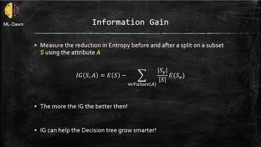
So, let me introduce you to all these little bits and pieces in the formula:
- E(S): The current entropy on our subset S, before any split
- |S|: The size or the number of instances in S
- A: An attribute in S that has a given set of values (Let’s say it is a discrete attribute)
- v: Stands for value and represents each value of the attribute A
- Sv: After splitting S using A, Sv refers to each of the resulted subsets from S, that share the same value in A
- E(Sv): The entropy of a subset Sv . This should be computed for each value of A (assuming it is a discrete attribute)
Could you tell me why we have that bloody ∑ over there? Well it is because the attribute A (let’s consider it a discrete attribute with N number of possible values) has N number of values and when we split using A, we need to compute the entropy for every branch corresponding to every value of A. The ∑ tries to sort of aggregate these individual entropy values after the split on A across all branches. Finally when we subtract the second term from E(S), we get the expected reduction in entropy if we choose attribute A for splitting. Cool ha? But we need a nice example to really understand it yes?
Consider the following nice dataset:
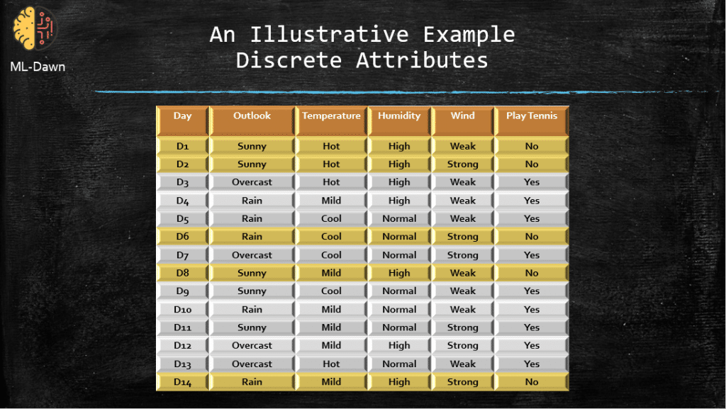
So we have a few attributes here, and the job is to learn when is Joe going to play tennis depending on the values these attributes can take. You can see that all of them these attributes are discrete and the target feature, Play Tennis, is actually both discrete and binary. The big question is, which attribute should we choose to learn whether Joe would play tennis on a given day? Outlook, Temperature, Humidity, or Wind?
Notice that all of these attributes are discrete but don’t worry, I will show you the big picture on how to compute IG for the continuous attributes as well. For now, let’s compute the IG for 2 of the attributes: Humidity and Wind and decide which one is a better candidate for splitting:
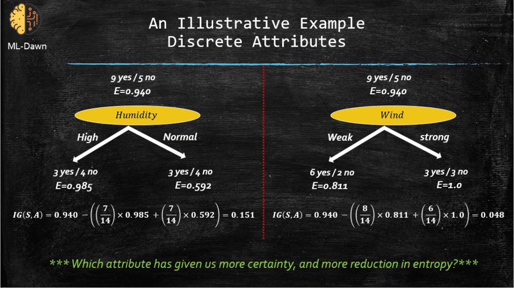
Beautiful! At the start, before the splitting started, we have and entropy of 0.94 which is quite high. Why? Because as I showed you before, in the case of binary classification the maximum of entropy for a given set S is always 1. So, 0.94 is pretty high! In the case of Humidity, the values are: High and Normal. On the left, for the case of value being equal to High, the |Sv|=7 (i.e., 3 yes / 4 no). Also, |S| is 14, as that is the number of samples in our subset before any splitting starts. So the question is, which attribute has given us more reduction in the initial entropy E(S) = 0.940. We can see that IG(S, Humidity) = 0.151 and it is larger than IG(S, Wind) = 0.048. As a result, the decision tree will choose Humidity over Wind for splitting. Simple, isn’t it?
So far all we have done has been on discrete attributes. Let’s consider our old dataset that has nothing but continuous attributes. Below, you can see the dataset and the corresponding decision tree, produced by Scikitlearn using Python.
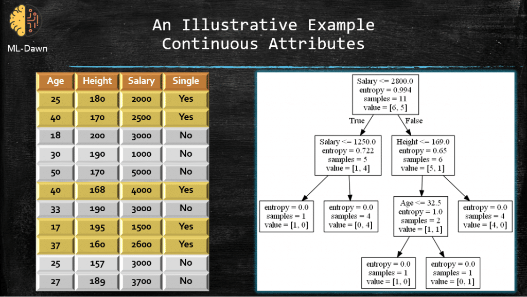
This is all nice and fun but there is a big question here:
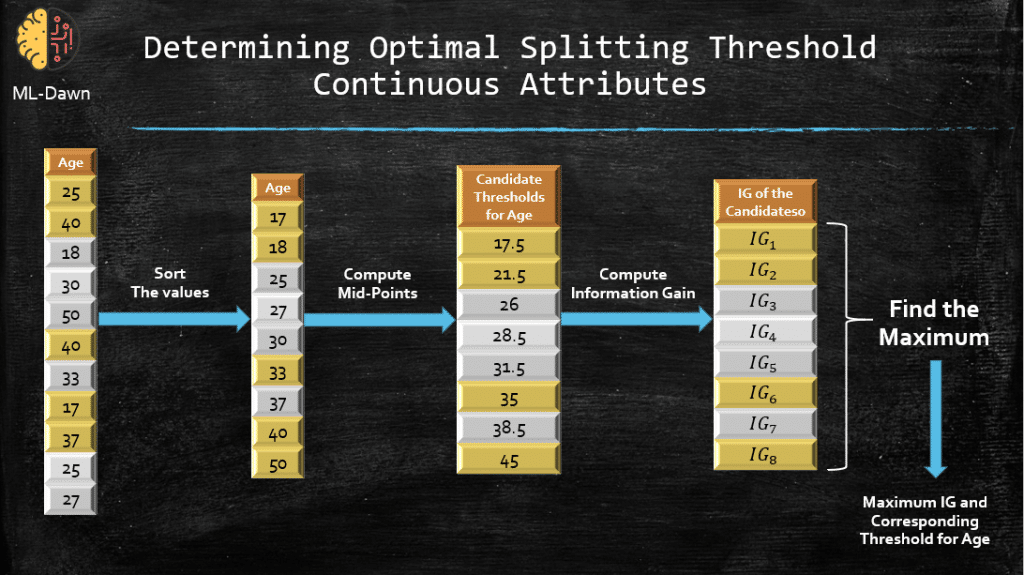
How does the DT decide on the threshold for the attributes to measure the reduction in entropy in the first place? For example, in the root of the tree we have a threshold of 2800.0 for Salary. But why?
It is actually quite simple. Let’s consider the Age attribute (the DT will do this for all the attributes). The question is: Which threshold for Age will give me the highest IG, that is, what is the best that Age can do in reducing the current entropy (E(S) = 0.994 which is too high)? Now, the DT first sorts the values of Age, and then considers the mid point for each pair of values. This becomes a vector of candidate threshold for the attribute Age. Now, the DT will measure the IG while splitting on Age using each and every value from the candidate threshold vector, and considers the highest IG and the corresponding candidate threshold. This will happen for all attributes, and the one with the highest IG with its corresponding threshold will be chosen for splitting. Below you can see the whole story for the attribute Age:
Weighted vs. Unweighted IG!
One of the most important features of Information Gain is how it aggregates the entropy values of multiple children nodes to report the final value for after the split on a given attribute. If you notice, what it does is actually a weighted averaging of the individual entropy values. It is weighted by the size of the subset per branch (Sv/S). This can be contrasted with a regular averaging that we all have learned when in high school, just so we can see why we have that weighted averaging.
For example, in our previous example where we split on Humidity, we got to branches with entropy values of 0.985 and 0.592. The way IG has mixed these two values is by weighting each one by |Sv |=7 over the original size of the subset before the split |S| = 14, that is 7/14=0.5. Now, why doesn’t IG just do a simple averaging and say (0.985 + 0.592)/2 ?
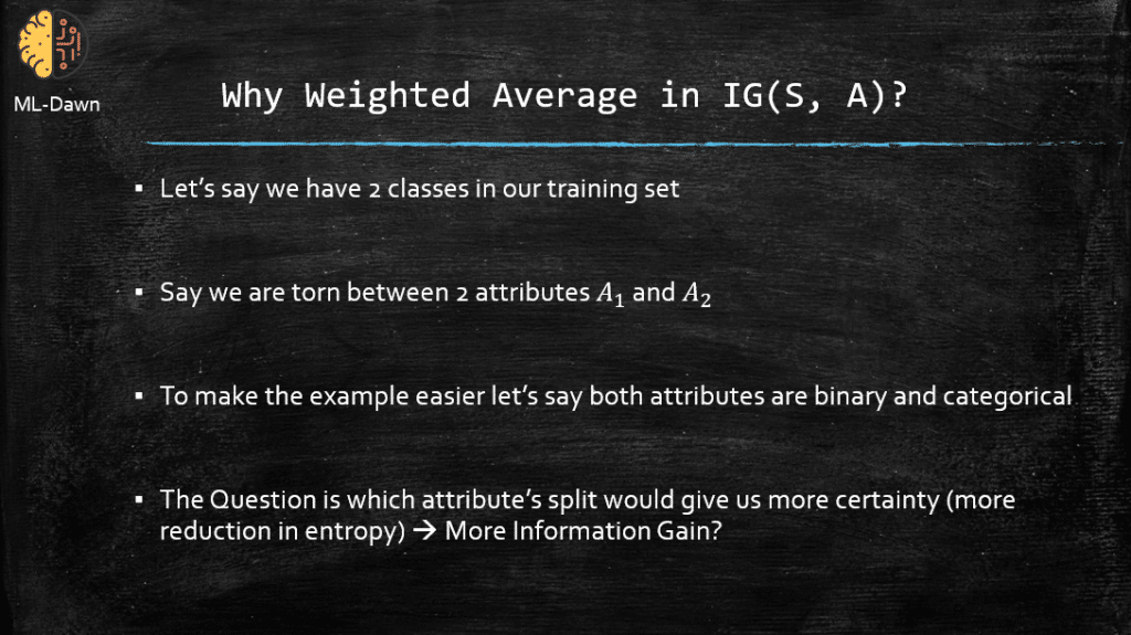
Now, take a look at 2 different splits and how a weighted and unweighted version of IG will report the best attribute for splitting.
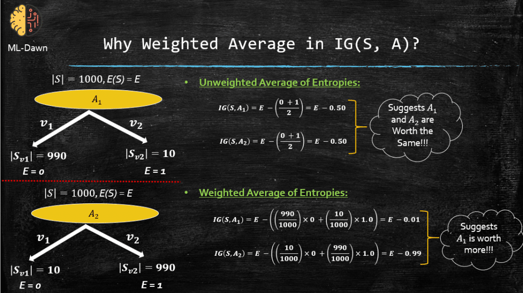
This is just really interesting! You can see that the unweighted version suggests that A1 and A2 are equally valuable, whereas the Weighted version, suggests that the split using A1 is almost 100 times better in terms of how much it reduces the entropy. This makes sense right? We can see this visually that:
The split on A1 has resulted in a HUGE chunk of pure set and a very small subset of non-pure.
However:
The split on A2 gives a very small pure subset and a HUGE impure subset.
It is clear that A1 must be rated better, which is determined correctly using the Weighted averaging that is done in IG. This is why they have bothered with the weighted averaging for IG and didn’t just do a simple averaging. Perfect!
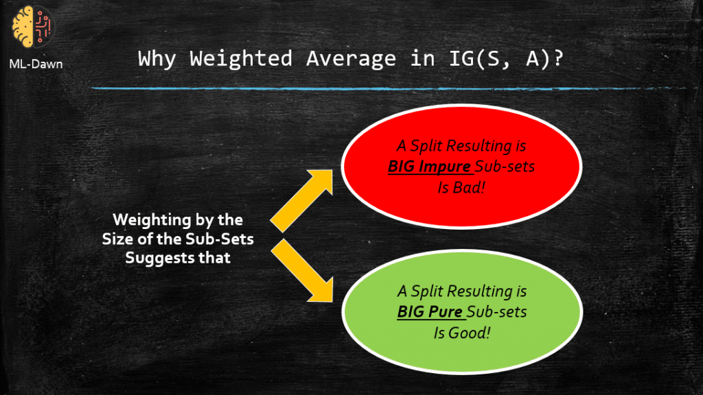
So the morals of the story as to why the weighted averaging is used can be summarized in the following:
Absolutely perfect! Now you know how a decision tree works. You know what entropy is an how Information Gain utilizes it to decide on the best attribute for splitting, for both discrete and continuous attributes. In the next post, we will talk about pruning and the techniques to avoid over-fitting to the training data.
Until then,
Take care of yourself,
MLDawn
Author: Mehran
Dr. Mehran H. Bazargani is a researcher and educator specialising in machine learning and computational neuroscience. He earned his Ph.D. from University College Dublin, where his research centered on semi-supervised anomaly detection through the application of One-Class Radial Basis Function (RBF) Networks. His academic foundation was laid with a Bachelor of Science degree in Information Technology, followed by a Master of Science in Computer Engineering from Eastern Mediterranean University, where he focused on molecular communication facilitated by relay nodes in nano wireless sensor networks. Dr. Bazargani’s research interests are situated at the intersection of artificial intelligence and neuroscience, with an emphasis on developing brain-inspired artificial neural networks grounded in the Free Energy Principle. His work aims to model human cognition, including perception, decision-making, and planning, by integrating advanced concepts such as predictive coding and active inference. As a NeuroInsight Marie Skłodowska-Curie Fellow, Dr. Bazargani is currently investigating the mechanisms underlying hallucinations, conceptualising them as instances of false inference about the environment. His research seeks to address this phenomenon in neuropsychiatric disorders by employing brain-inspired AI models, notably predictive coding (PC) networks, to simulate hallucinatory experiences in human perception.




Responses