
Initialize each learnable parameter
to a small random value
Until the termination condition is met, do
For each pair of training example (
,
), do:
Feed
Update each learnable parameter
In the above algorithm, , represents a given input data—It can have a certain dimensionality,
. And
represents the ground truth for the given input data. This is what the model strives to learn to predict! Here is something that might not strike you at first glance:
For every single input data,
What?! Hell yeah! I am going to show you how this happens.
In this section, I would like to define a model, that takes 1 scalar input, , and has 1 trainable parameter,
. By linearly combining them, the model produces the output
. Finally, I will define a loss function that takes the output of the model and computes the loss. For simplicity, this particular loss function does not need the ground-truth,
. This can happen in an unsupervised learning scenario!
I am sick of seeing that bloody bowl-shaped loss surface in every single machine learning book and blog (including my own blog)! Even though it is legit, I want to define a highly convex loss surface with loads of local minima and maxima. I want you to see how SGD will walk out of all of these traps and finds the global minimum!
So, let’s define our model’s output as a function of the input and the trainable weight parameter:
and our loss is computed as follows:
I know, it is a funny looking loss! I will show you how it looks like in the hypothesis space of possible values for our parameter . Of course, we will need to take the derivative of this loss with respect to our trainable parameter,
, so that SGD could actually update
, while minimizing the loss as fast as possible. So, this is the only mathematically heavy part of this post (I promise!):
From the Chain-Rule we know that:
And also, remember the multiplication rule for computing derivatives:
So, let’s first compute :
Using the multiplication rule, we have:
And we know that . I will leave the rest of the algebraic hassle to you (I believe in you ;-)), however, your final answer should be this:
Enough with the math! Let’s dive into some cool visualizations and some nice Python code.
Let’s now code the 2 most important functions. First one computes the loss for a given model output, . The second one, computes the derivative of the loss w.r.t the parameter
, given an input data,
:
We know that our loss function is a function of the input data, , and the learnable parameter,
. Given an input data, we can actually plot this surface! What is the name of this surface? It is actually the hypothesis space and the corresponding loss value for every value of the parameter
, in that space:
The hypothesis space, is the space of all possible values for our learnable parameters. In our case, this is a space of scalar values for our one and only learnable parameter,
! We would like to search in this space, and find a value for
Let’s take a look at some of the loss surfaces, given a few of the training data. For each training example, we will go over a grid of possible values of , and compute the loss for each value of
, given the fixed value of the input data.
If we have
input data, we will have
The following code produces 3 input data, and plots 3 loss surfaces for us, across the hypothesis space of .

I would like to show you, a 3-dimensional view of many of such surfaces! In other words, a visualization across a range of values for the input data , and the learnable parameter,
and the computed loss value corresponding to each pair of (
,
)! This shows you how much indeed, can the loss surface change, with even a small change in the value of
! The code below, creates a grid of values for
and
, computes the loss for each pair of (
,
) and visualizes a 3-dimensional plot:


A very important point:
SGD will NOT take place on this 3D surface! Note that this is NOT our hypothesis space! For a given input data
Perfect! Now we are going to do something really cool! We will define a dataset of scalar values, and feed each one into our model, produce the model output, and compute the loss. Then compute the gradient at a particular weight value and compute the new value for
, and call it
. By computing the corresponding loss value for
and
, we basically have the coordinates of the start and the end of the update vector for our parameter,
.
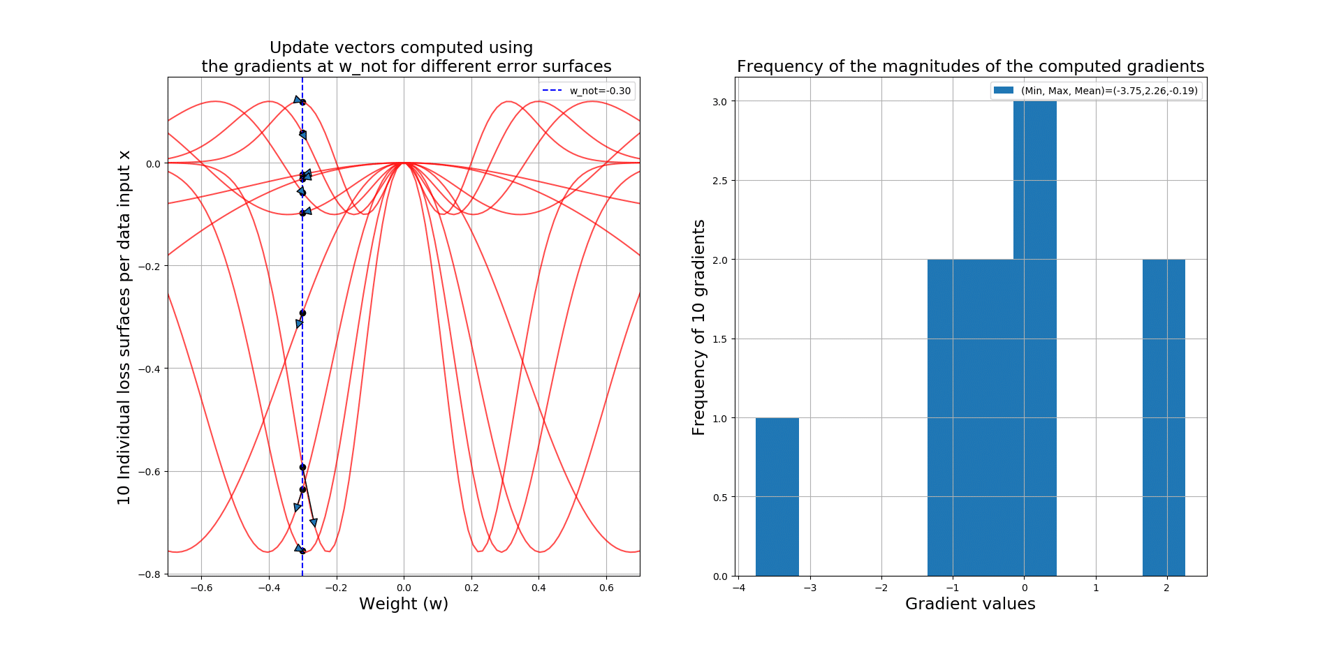
Given each data point, at point , we will compute a different gradient value, since the loss surface changes for every input example! So, if we have 100 input data, then we will have 100 loss surfaces, and 100 gradient values at
across all 100 loss surfaces. Using a histogram, we can gain some insight into the magnitudes of these gradients regarding their distribution, and some statistics like the minimum, maximum and average of them.
So when you hear people saying SGD is really noisy, it is because of the fact that, for every input data, you will have a different error surface and gradient, which you will use to update your parameters! However, this noise can be really helpful, to help you JUMP OUT of the local minima! In other words, it will literally KICK you OUT of the local minima with the hope that you could find the global minimum (i.e., -0.76 in our example).
Let’s take a look at the code that will generate 10 loss surfaces, plots the update vector starting at and ending in
:


Here is the reward for all of you who have survived this far! Let’s apply the SGD algorithm, and search the hypothesis space for the best value for our learnable parameter , so that hopefully we could find the global minimum 0.76. The main part to focus on in the code below is that:
For every input data, after computing the gradient at current
, we will UPDATE
Let’s travel with SGD on many loss surfaces and see how we will occasionally get trapped at some local minima but SGD, due to its stochasticity (where for EVERY data point we have a different loss surface), kicks us out of those minima! See how this will help us find the global minimum! The code below, initiates SGD and the travel in the hypothesis space:


Responses