Train a Perceptron to Learn the AND Gate from Scratch in Python

What will you Learn in this Post?

Neural Networks are function approximators. For example, in a supervised learning setting, given loads of inputs and loads of outputs in our training data, a neural network is capable of finding the hidden mapping between the those inputs and outputs. It can also, hopefully, generalize its acquired knowledge to the unknown and unseen data in the future.

One particular type of such functions is the boolean functions such as, AND, OR, NAND, NOR, XOR, … . In this post you will learn how to code a neural network (A perceptron) to learn a boolean function and you will see where a simple perceptron will fail!

The Representative Power of a Perceptron

So, a perceptron shown below, is capable of learning decision boundaries in a binary classification scenario. For example, if your inputs are 1-Dimensional or 2-Dimensional, we can actually visualize different parts of our perceptron. Below, in the 1-Dimensional case you can see how the input and the bias unit are linearly combined using the weights, resulting in Z. Then you can see that we apply the thresholding function on top of Z to create our binary classifier. This classifier outputs +1 for instances of one class, and -1 for the instances of the other class.

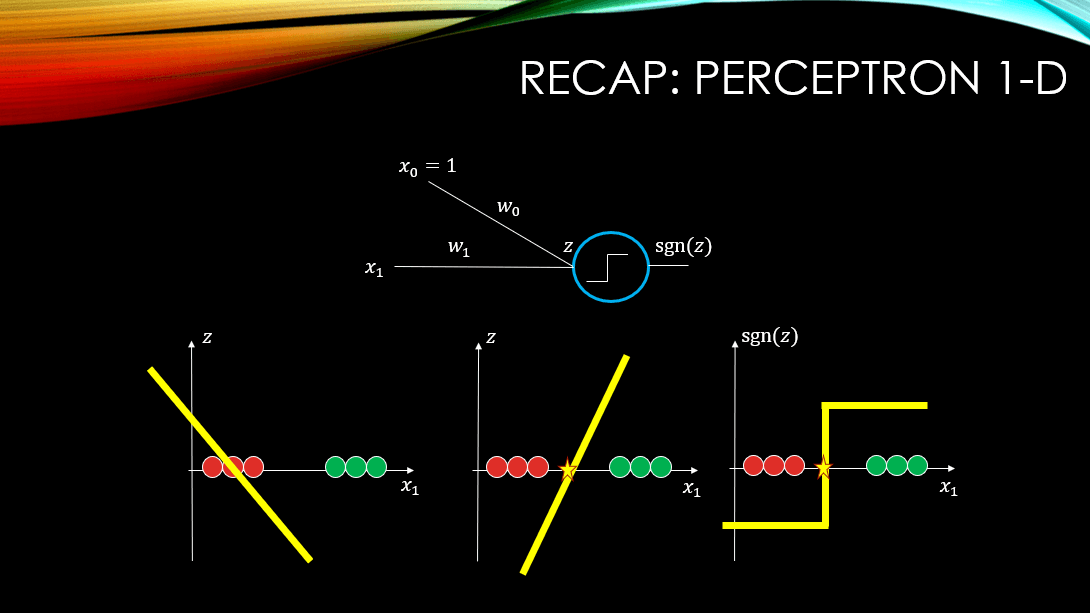
The sgn(Z) is our sign function where if Z>0, outputs +1 and if Z<0, it outputs -1. You notice how when our input data is 1-Dimensional, our Z is a 2-Dimensional figure namely a line:  . However, our decision boundary, where Z cuts through our input space (i.e., where Z=0), is a point and it is 1-Dimensional just like our input data. What about a 2-Dimensional input data? What will Z be then?

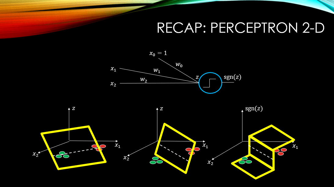
Our input data is 2-Dimensional but note that our Z is now a plane: . So, our input space is 2-Dimensional but our Z is 3-Dimensional! See what happens when Z cuts through our input space ( plane)! The result is a line (again a 2-Dimensional shape) that is our decision boundary and it is where Z=0. Again by applying sgn(Z) on Z we can generate +1/-1 for the instances the 2 classes in our dataset!

Now, let’s refresh our minds on boolean functions and then see how we can learn such function using our perceptron 😉

Boolean Functions (A Reminder)

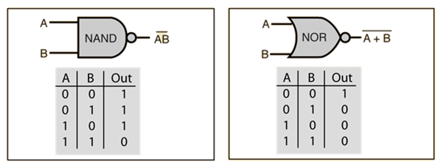
So, boolean functions, at least the main ones can be summarized, below:

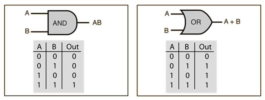
Make no mistake! These are functions as well! We have inputs and we have outputs! So, for example the AND gate’s logic, from a human’s perspective is:

The output of the AND gate is +1 if and only if all of its inputs are positive (greater than 0), and the output is 0, if at least there is one non-positive input to the gate!

But a machine has no idea about this logic! We want to see whether we can train a machine learning algorithm, namely, a simple perceptron, to learn such gates.

Linearly Separable Gates and Perceptrons

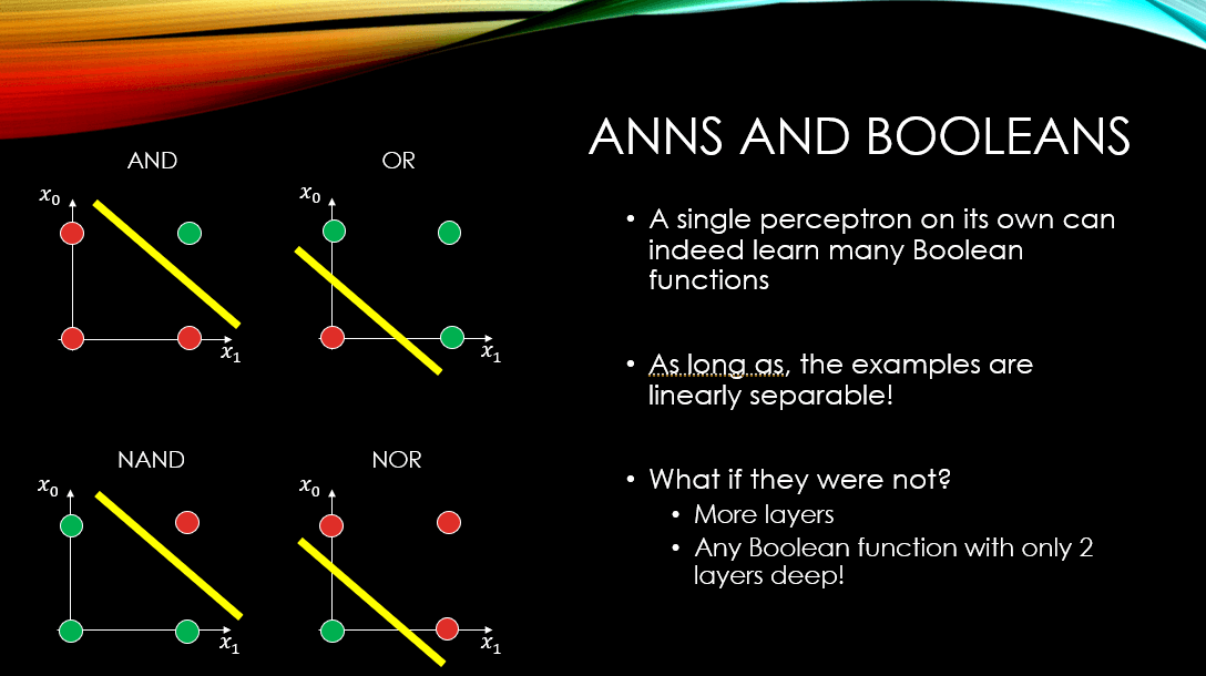
If we look at the 2-Dimensional input space of boolean functions, and color positive examples with green and negatives with red, then we can visualise our training data like below. Note that, the yellow line is a decision boundary that can separate the 2 classes beautifully, and hopefully our neural network will be able to find such a boundary!

It is important to note that not all gates can be learned by a single perceptron! For instance the XOR gate, represented below, can NEVER EVER be learned by a single perceptron! Why?

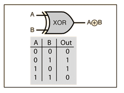
In order to see why, I have to remind you that:

A single perceptron can learn any function, as long as the instances in the dataset are linearly separable, like AND, OR, NAND, and NOR!

Now what about the XOR?

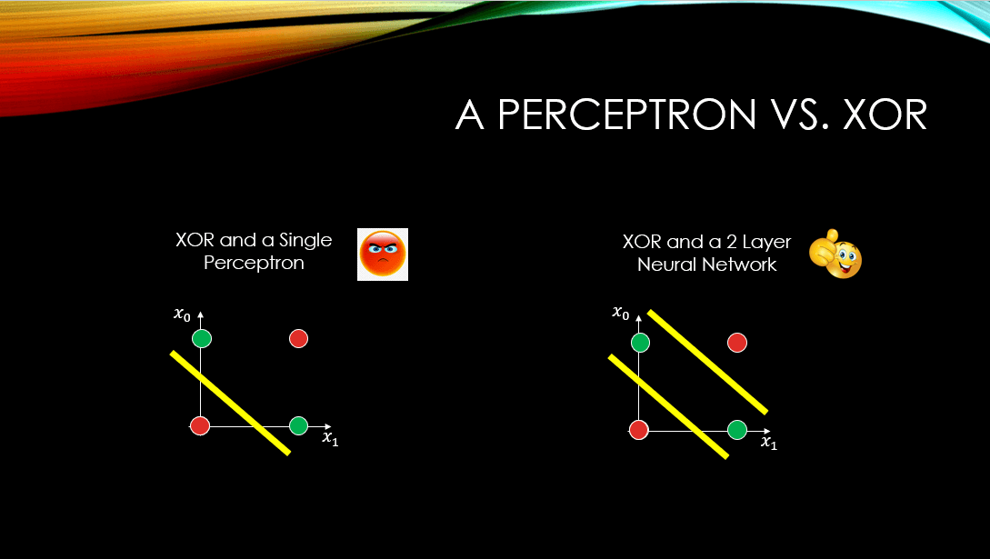
In the image above, it is clear that the positive and negative examples are not linearly separable, so a perceptron can never find any line to separate them (The image on the left). However, if only we had a neural network with at least 2 layers of depth, we could separate these examples (The image on the right).

Teaching a Perceptron the AND Gate (CODE)

Of all the gates that are linearly separable, we have chosen the AND gate to code from scratch. First foremost, let’s take a look at our perceptron:

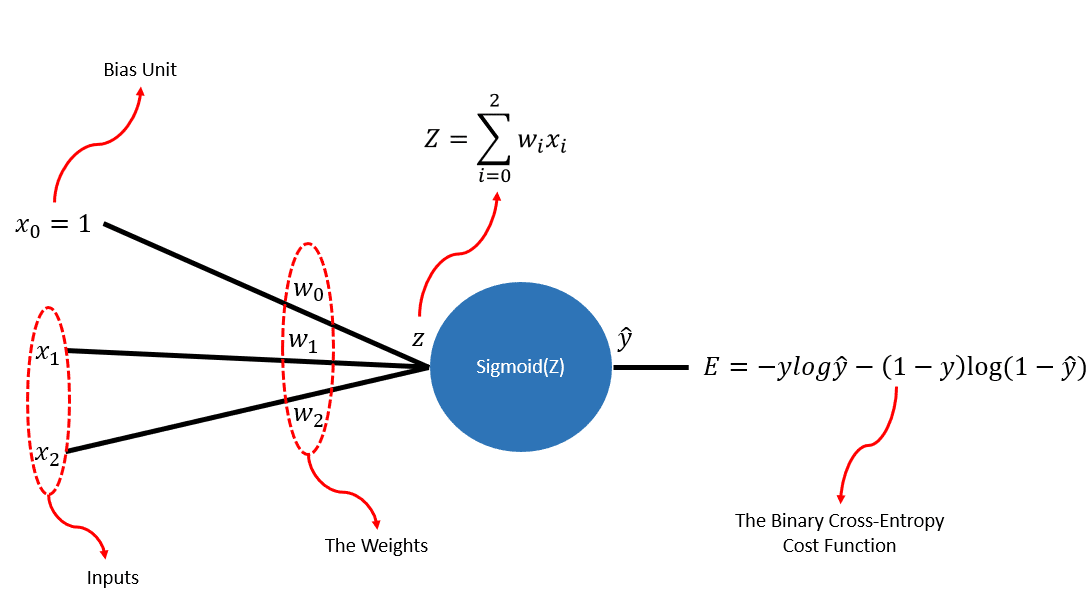
Now you notice that I have used the sigmoid() function, instead of a step function. The reason is that during back-propagation, we need all the functions that we have used during the forward pass to be differentiable! Now, the step function is not differentiable as it breaks at point 0 (when its input is 0)! So, I have used the sigmoid() function, which is differentiable all across and is continuous!

Now, we need to import these packages :

# Numpy is used for all mathematical operations
import numpy as np
# For plotting purposes
import matplotlib.pyplot as plt
from mpl_toolkits.mplot3d import axes3d # 3 Dimensional plotting
from matplotlib import cm # For some fancy plotting ;-)

I am sure that as a Neural Network enthusiasts, you are familiar with the idea of the sigmoid() function and the binary-cross entropy function. We need to use them during the forward-pass. Before showing you the code, let me refresh your memory on the math: and as for the binary-cross entropy: 

Note that: The base of the logarithm is e. Meaning that what we have here is the Natural Logarithm!

Remember that this error function is nothing but a measure of difference between the output of the ANN, , and the ground-truth, y. So, the lower it is, the better (of course not to the point of over-fitting to the training data 😉 )!

Now let’s see the code.  We can code both of these 2 functions using 2 separate python functions in Python:

def Cross_Entropy(y_hat, y):
    # There are 2 possibilities for the ground-truth: either 0 or 1
    # Note that np.log() is actually the natural logarithm with e, for its base
    if y == 1:
      return -np.log(y_hat)
    else:
      return -np.log(1 - y_hat)
# This is just the classic sigmoid function, given input z
def sigmoid(z):
    return 1 / (1 + np.exp(-z))

Now, we have to think ahead, right? So, during the back-propagation phase, we will need 2 things!

1. The derivative of the Error w.r.t the output

2. The derivative of the output w.r.t  Z (i.e., the derivative of the output of the sigmoid() function w.r.t the input of the sigmoid() function that is, Z)

Now, as a reminder:

And as for the sigmoid(z), or for short, sig(z):

This is not a neural network course, so I am not going to derive these here mathematically and step by step. Now, let us code the 2 functions in Python, whose job is to compute these derivatives:

def derivative_Cross_Entropy(y_hat, y):
    # Again we account for 2 possibilities of y=0/1
    if y == 1:
      return -1/y_hat
    else:
      return 1 / (1 - y_hat)
# The derivative of sigmoid is quite straight-forward
def derivative_sigmoid(x):
    return x*(1-x)

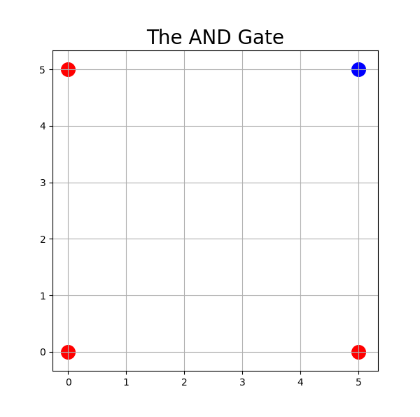
Now, let’s build our dataset. We start wtih the AND gate. Remember: AND returns 1 if and only if all of its inputs are positive.

# Our data
X = np.array([[0, 0], [0, 5], [5, 0], [5, 5]])
# The ground truth (i.e., what AND returns and our perceptron should learn to produce)
Y = np.array([0, 0, 0, 1])

Let’s also visualise our dataset using the following code:

The size of each data point
area = 200
fig = plt.figure(figsize=(6, 6))
plt.title('The AND Gate', fontsize=20)
ax = fig.add_subplot(111)
# color red: is class 0 and color blue is class 1.
ax.scatter(0, 0, s=area, c='r', label="Class 0")
ax.scatter(0, 5, s=area, c='r', label="Class 0")
ax.scatter(5, 0, s=area, c='r', label="Class 0")
ax.scatter(5, 5, s=area, c='b', label="Class 1")
plt.grid()
plt.show()

First, we need to initialise our weights, of which we need 3:

# We consider a low and high range for our random weight generation
# Remember we consider this rage to be small, so that during the back-propagation
# Our gradients through the sigmoid unit will stay strong. This is a major concern in
# Deep nets however!
low = -0.01
high = 0.01
# We are using uniform distribution for our random weight generation.
W_2 = np.random.uniform(low=low, high=high, size=(1,))
W_1 = np.random.uniform(low=low, high=high, size=(1,))
W_0 = np.random.uniform(low=low, high=high, size=(1,))

Also, let’s determine the number of epochs, and the learning rate:

# Number of our epochs. Every epoch is a complete sweep through our data
Epoch = 2000
# The learning rate. Preferably a small value!
eta = 0.01

Finally, the big monster is here. Let’s start the training phase:

# E will contain the average cross-entropy error per epoch
E = []
# The actual training starts for as many times as Epoch.
for ep in range(Epoch):
    # Shuffle the train_data X and its Labels Y. Almost always a good practice to shuffle in the beginning of the epoch! 
    random_index = np.arange(X.shape[0])
    # Now random_index has the same length as X and Y, and contains a shuffled index list for X. 
    np.random.shuffle(random_index)
    # e will record errors in an epoch. Then will be averaged, and this average value will be added to E.
    # We reset e[], in the beginning of each epoch
    e = []
    # This loop goes through the shuffled training data. random_index makes sure for training data 
    # in X we are grabbing the correct ground truth from Y
    for i in random_index:
        # Grab the ith training data from X
        x = X[i]
        # Compute Z, which is the input to our sigmoidal unit
        Z = W_1* x[0] + W_2* x[1] + W_0
        # Apply sigmoid, to produce an output by the perceptron
        Y_hat = sigmoid(Z)
        # Compute the binary cross-entropy error for this ith data point and add it to e[]
        e.append(Cross_Entropy(Y_hat, Y[i]))
        # Compute the gradients of our error function w.r.t. all 3 learnable parameters (i.e., the weights of our network)
        dEdW_1 = derivative_Cross_Entropy(Y_hat, Y[i])*derivative_sigmoid(Y_hat)*x[0]
        dEdW_2 = derivative_Cross_Entropy(Y_hat, Y[i]) * derivative_sigmoid(Y_hat) * x[1]
        dEdW_0 = derivative_Cross_Entropy(Y_hat, Y[i])*derivative_sigmoid(Y_hat)
        # Update the parameters using the computed gradients. So, we update after each individual data point => Stochastic gradient descent!
        W_0 = W_0 - eta * dEdW_0
        W_1 = W_1 - eta*dEdW_1
        W_2 = W_2 - eta* dEdW_2
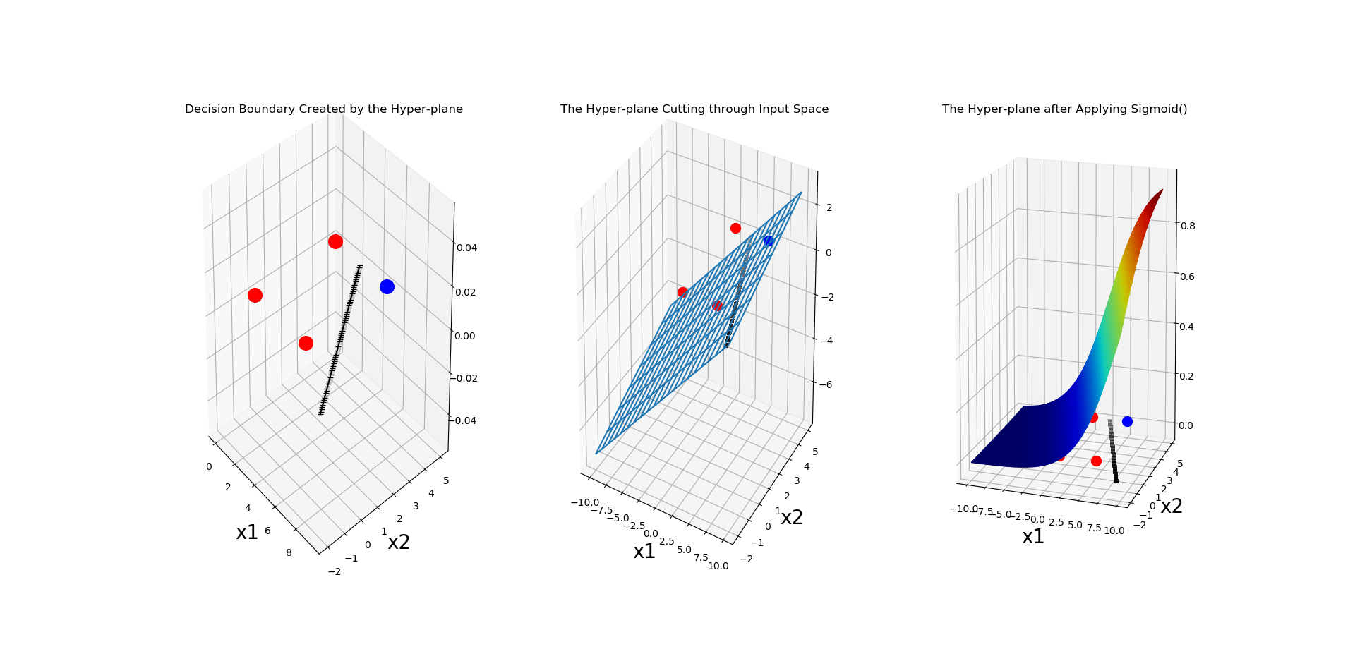
    # Every 500 epochs, we would like to visualise 3 things: 1) The linear 2-Dimensional decision boundary in the input space
    # 2) The actual hyper-plane in the 3-Dimensional space, which by cutting through the input space, 
    # has produced our linear decision boundary, which is the same as our Z (i.e., the input to our sigmoidal unit).
    # Finally, the sigmoid() of this Z, which should squash the hyper-plane between 0 and 1, by definition. NOTE: sigmoid(Z) always 
    # squashes Z into a value in the range [0, 1]
    if ep % 500 == 0:
        # Generate a figure
        fig = plt.figure(figsize=(6, 6))
        plt.title('The AND Gate', fontsize=20)
        # Insert a sub-figure and make sure it is capable of 3-Dimensional rendering
        ax = fig.add_subplot(131, projection='3d')
        # Plot individual data points in this sub-figure
        ax.scatter(0, 0, s=area, c='r', label="Class 0")
        ax.scatter(0, 5, s=area, c='r', label="Class 0")
        ax.scatter(5, 0, s=area, c='r', label="Class 0")
        ax.scatter(5, 5, s=area, c='b', label="Class 1")
        # Give a title to this sub-figure
        plt.title('Decision Boundary Created by the Hyper-plane')
        # The equation of Z = W2X2 + W1X1 + W0 and we know that the linear decision boundary's equation is obtainable by setting Z = 0
        # So, W2X2 + W1X1 + W0 = 0, and by rearranging: x_2 = (-W1/W2) * x1 - (W0/W2) which is a line with the slope (-W1/W2) and the
        # intercept - (W0/W2). Note that the weights are being learned by the perceptron, however, we choose a range of values for x1, 
        # and for each we compute x2. Why a range? because we want to plot a continuous line here, and our x's are just discrete values
        # That can be either 0 or 5 (as shown in our dataset.) 
        x_1 = np.arange(-2, 5, 0.1)
        W_1 * x[0] + W_2 * x[1] + W_0
        x_2 = (-W_1/W_2) * x_1 - (W_0/W_2)
        plt.grid()
        plt.plot(x_2, x_1, '-k', marker='_', label="DB")
        plt.xlabel('x1', fontsize=20)
        plt.ylabel('x2', fontsize=20)
        # Now we add the second sub-figure. This well wisualize the hyper-plane X and the way it cuts through the input space
        ax = fig.add_subplot(132, projection='3d')
        x_0 = np.arange(-10, 10, 0.1)
        # we need a mesh-grid for 3-Dimensional plotting
        X_0, X_1 = np.meshgrid(x_0, x_1)
        # for every combination of points from X_0 and X_1, we generate a value for Z in 3-Dimensions
        Z = X_0*W_1 + X_1*W_2 + W_0
        # We use the wire_frame package so we could see behind this hyper-plane. The stride arguements, 
        # determine the grid-size on this plane. The smaller their values, the finer the grid on the hyper-plane
        ax.plot_wireframe(X_0, X_1, Z, rstride=10, cstride=10)
        # We still want to visualize the linear decision boundary computed in the previous sub-figure
        ax.scatter(x_2, x_1, 0, marker='_', c='k')
        # Again plot our data points as well for this sub-figure
        ax.scatter(0, 0, 0, marker='o', c='r', s=100)
        ax.scatter(0, 5, 0, marker='o', c='r', s=100)
        ax.scatter(5, 0, 0, marker='o', c='r', s=100)
        ax.scatter(5, 5, 0, marker='o', c='b', s=100)
        plt.xlabel('x1', fontsize=20)
        plt.ylabel('x2', fontsize=20)
        plt.title('The Hyper-plane Cutting through Input Space')
        plt.grid()
        # Add the last sub-figure that will show the power of sigmoid(), and highlights how Z gets squashed between 0 and 1
        ax = fig.add_subplot(133, projection='3d')
        # This is really cool! The cm package will color the figure generated by sigmoid(Z), based on the value of sigmoid(Z).
        # Brighter colors are closer to 1 and darker ones are closer to 0! This way you can see how the sigmoid(Z), which is the final
        # Output of our perceptron y_hat, will assign values closer to 1 for our positive examples and values closer to 0 for our negative
        # examples.
        my_col = cm.jet(sigmoid(Z) / np.amax(sigmoid(Z)))
        ax.plot_surface(X_0, X_1, sigmoid(Z), facecolors=my_col)
        # Again we want to see the linear decision boundary produced in the first sub-figure with our actual training examples
        ax.scatter(x_2, x_1, 0, marker='_', c='k')
        ax.scatter(0, 0, 0, marker='o', c='r', s=100)
        ax.scatter(0, 5, 0, marker='o', c='r', s=100)
        ax.scatter(5, 0, 0, marker='o', c='r', s=100)
        ax.scatter(5, 5, 0, marker='o', c='b', s=100)
        plt.title('The Hyper-plane after Applying Sigmoid()')
        plt.xlabel('x1', fontsize=20)
        plt.ylabel('x2', fontsize=20)
        plt.grid()
        plt.show()
    # Now e has the errors for every training example in our training set through out the current epoch. We average that and add it to E[]
    E.append(np.mean(e))

Here is one of the outputs generated after 500 epochs:

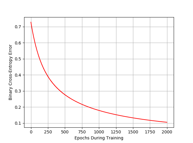
And let’s also plot the error values that we have been recording, per epoch:

plt.figure()
plt.grid()
plt.xlabel("Epochs During Training")
plt.ylabel("Binary Cross-Entropy Error")
plt.plot(E, c='r')
plt.show()

I Have 2 Challenges for You !!!

1) Can you modify the code in a way that the training data would correspond the XOR gate? 

The network should NEVER converge as there is no way for a line to separate linearly inseparable examples! The error function should look something nasty and non-converging like this:

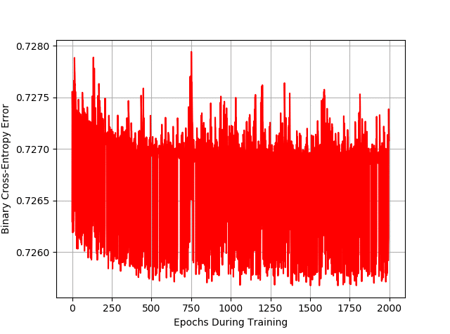
The error is almost never going down! See if you can generate this!

2) See if by coding a 2-layer neural network you could learn the XOR gate?

Feel free to post your findings and outputs in the comments.

I do hope that you have enjoyed this post and it has been informative for you,

Regards,

MLDawn

Author: mehran@mldawn.com

Dr. Mehran H. Bazargani is a researcher and educator specialising in machine learning and computational neuroscience. He earned his Ph.D. from University College Dublin, where his research centered on semi-supervised anomaly detection through the application of One-Class Radial Basis Function (RBF) Networks. His academic foundation was laid with a Bachelor of Science degree in Information Technology, followed by a Master of Science in Computer Engineering from Eastern Mediterranean University, where he focused on molecular communication facilitated by relay nodes in nano wireless sensor networks. Dr. Bazargani’s research interests are situated at the intersection of artificial intelligence and neuroscience, with an emphasis on developing brain-inspired artificial neural networks grounded in the Free Energy Principle. His work aims to model human cognition, including perception, decision-making, and planning, by integrating advanced concepts such as predictive coding and active inference. As a NeuroInsight Marie Skłodowska-Curie Fellow, Dr. Bazargani is currently investigating the mechanisms underlying hallucinations, conceptualising them as instances of false inference about the environment. His research seeks to address this phenomenon in neuropsychiatric disorders by employing brain-inspired AI models, notably predictive coding (PC) networks, to simulate hallucinatory experiences in human perception.