
Neural Networks: Artificial neural networks have been investigated and applied to the famous MNIST dataset and the test risk is computed as opposed to the capacity of the neural network. In particular, they have used a single layer fully-connected neural network with hidden units, where the number of parameters (i.e., weights) are used to increase the capacity of the model. This is a classification task, and the job is to learn to classify hand-written digits into their corresponding correct classes, of which we have 10, one for each digit: 0,1,2,…,9. In this case, the number of data samples are
, the dimensionality of the data,
, is 784 (remember: the images in MNIST are 28×28 pixel which amounts to 784 pixel values), and the number of classes,
, is 10. The number of parameters is then
. The reason for adding 1 in this formula is that in both the input layer and the hidden layer there is an additional bias unit. The interpolation threshold (black dotted line) is observed at
.
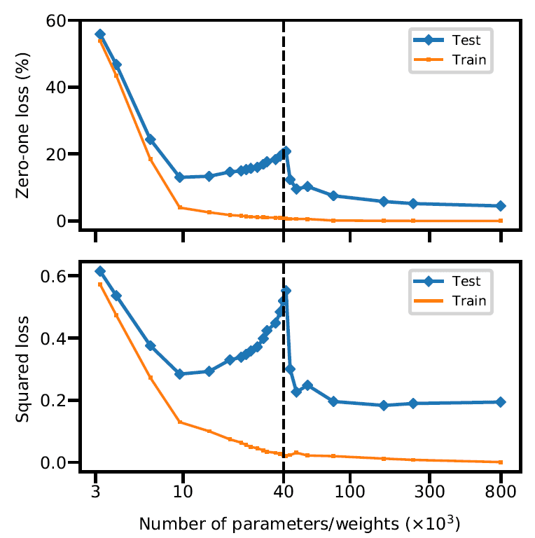
It is absolutely astonishing that we can see how the double-descent is happening right before our very eyes! This happens whether a simple Zero-loss or the squared loss is used!
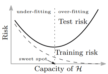
However, what structural mechanisms, as the authors put it, account for the double descent shape?
This has something to do with the number of features, and the number of data instance,
. When the number of features is much smaller than the number of data instances (i.e.,
), the training and test risks are close. This is where by adding more features (i.e., increasing
) the performance on both train and test sets will improve. However, as the number of features approach the number of data instances (this is the interpolation point
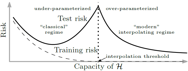
), the test risk is at its peak which means we are maximally over-fitting! This is where, we have increased the number of features to a point where some features that are not present in the data (or even weakly present) are forced to fit the training data almost perfectly. However, the authors kept on pushing and increased the number of features beyond the interpolation point! By increasing the number of features, a better and better approximations to that smallest norm function (i.e., the simplest and smoothest function) can be constructed.
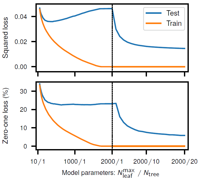
Random Forests: The same experiment as before is done, however, using a random forest model this time. The double descent risk curve is observed for random forests with increasing model complexity trained on MNIST ( = 104; 10 classes). Its complexity is controlled by the number of trees
and the maximum number of leaves allowed for each tree
.

Author: Mehran
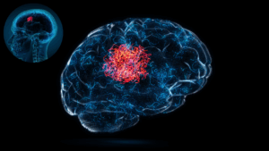
Dr. Mehran H. Bazargani is a researcher and educator specialising in machine learning and computational neuroscience. He earned his Ph.D. from University College Dublin, where his research centered on semi-supervised anomaly detection through the application of One-Class Radial Basis Function (RBF) Networks. His academic foundation was laid with a Bachelor of Science degree in Information Technology, followed by a Master of Science in Computer Engineering from Eastern Mediterranean University, where he focused on molecular communication facilitated by relay nodes in nano wireless sensor networks. Dr. Bazargani’s research interests are situated at the intersection of artificial intelligence and neuroscience, with an emphasis on developing brain-inspired artificial neural networks grounded in the Free Energy Principle. His work aims to model human cognition, including perception, decision-making, and planning, by integrating advanced concepts such as predictive coding and active inference. As a NeuroInsight Marie Skłodowska-Curie Fellow, Dr. Bazargani is currently investigating the mechanisms underlying hallucinations, conceptualising them as instances of false inference about the environment. His research seeks to address this phenomenon in neuropsychiatric disorders by employing brain-inspired AI models, notably predictive coding (PC) networks, to simulate hallucinatory experiences in human perception.


Responses