Linear Regression from Scratch using Numpy

Home

/

Linear Regression from Scratch using Numpy

Hello friends and welcome to MLDawn!

So what sometimes concerns me is the fact that magnificent packages such as PyTorch (indeed amazing), TensorFlow (indeed a nightmare), and Keras (indeed great), have prevented machine learning enthusiasts to really learn the science behind how the machine learns. To be more accurate, there is nothing wrong with having these packages but I suppose we, as humans, have always wanted to learn the fast and easy way! I am arguing that while we enjoy the speed and ease of coding that such packages bless us with, we need to know what is happening behind the scene!

For example, when we want to build a complicated multi-class classifier with a sophisticated Artificial Neural Network (ANN) architecture, full of convolutional layers and recurrent units, we need to ask ourselves:

Do I know the logic behind this?! Why convolutional layers? Why recurrent layers? Why do I use a softmax() function as the output function? And why do people always use cross-entropy as the appropriate error function in such scenarios? Is there a reason why cross-entropy pairs well with softmax?

So, one way we could understand the answer to some of these questions, is to see whether we can implement a simple Neural Network, say a simple regression model, on some synthetic 1-dimensional data using the simplest ANN possible, from scratch!

In this post we will code this simple neural network from scratch using numpy! We will also use matplotlib for some nice visualisations.

So, if we consider our synthetic data to be a bunch of scalars, and 1-Dimensional, this is the simple ANN structure that we could be interested in building from scratch!

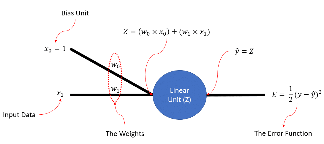
So, as we can see in the figure, $Z$ is simply the linear combination of the input $x_1$ and the bias unit $x_0$ . Then we have a linear unit (i.e., linear neuron) that literally does nothing, but I have put it there so the whole network would look like a neural network. Moreover, $y_{hat}$ , that is the output of our neural, is exactly equal to $Z$ , because the neuron is linear. Finally, we have the error function, $E$ , that actually has a name: Sum Squared Error (SSE).

Right! So, now it is time to do the coding bit. First foremost, let’s import the necessary packages! The almighty numpy and matplotlib’s pyplot are both needed.

# Import numpy for all mathematical operations and also generating our synthetic data
import numpy as np
# Matplotlib is going to be used for visualisations
import matplotlib.pyplot as plt

I am sure that as a Neural Network enthusiast, you are familiar with the idea of the Linear() function and the sum squared error function. We need to use them during the forward-pass phase of training our ANN. Before showing you the code, let me refresh your memory on the math. So, the Linear() function can be defined as:

$Linear(X)=X$

And the sum squared error for ground-truth $y$ and prediction $y_{hat}$ , can be defined as:

$E(y, y_{hat}) = \frac{1}{2}(y - y_{hat})^2$

Remember that this error function is nothing but a measure of difference between the output of the ANN, $y_{hat}$ , and the ground-truth, $y$ . So, the lower this error is the better!

Now let’s see the code. We can code both of these 2 functions using 2 separate python functions:

# The sum squared error (SSE)
def SSE(y, y_hat):
    return 0.50*np.sum((y- y_hat)**2)
# The linear function
def Linear(Z):
    return Z

As you notice, we have a summation operation is the SSE() function. Why? Because we are doing batch learning, which means that given all of our training data, $X$ , we will have a prediction for all of them, $y_{hat}$ , and a ground-truth, $y$ , for each and every one of them.

So, in the SSE() error function, $y$ and $y_{hat}$ are vectors. If our training data $X$ has the size of $N$ , then both $y$ and $y_{hat}$ also have the size $N$ . In batch-learning, we feed ALL our training set $X$ into our ANN, and produce all the predictions, in one go! So, we need to sum the errors of individual errors for each input data, hence the use of np.sum() in the SSE() function above!

Now, we have to think ahead, right? So, during the back-propagation phase, we will need 3 things:

The derivative of the error, $E$ , w.r.t our output, $y_{hat}$ :

$\frac{dE}{dy_{hat}} = y_{hat} - y$ The derivative of our output, $y_{hat}$ , w.r.t $Z$ : $\frac{dy_{hat}}{dZ} = 1$ The derivative of $Z$ , w.r.t. $w_0$ and $w_1$ :

$\frac{dZ}{dw_1} = x_1$ and $\frac{dZ}{dw_0} = x_0 = 1$

In other words, using the chain rule, we can compute the derivative of our error function w.r.t. both of our learnable parameters $w_0$ and $w_1$ : $\frac{dE}{dw_1} = \frac{dE}{dy_{hat}}\times \frac{dy_{hat}}{dZ} \times \frac{dZ}{dw_{1}}$

$\frac{dE}{dw_1} = -(y-y_{hat})\times1\times x_1 = -(y-y_{hat})\times x_1$

$\frac{dE}{dw_0}= -(y - y_{hat})\times 1 \times x_0 = -(y - y_{hat})$

You notice that $x_0$ is eliminated, as we know that it is the bias unit and $x_0 = 1$ .

So, let’s define 2 functions for computing both derivatives:

def dEdW_1 (y, y_hat,x_1):
    return np.sum(-(y - y_hat) * x_1)

def dEdW_0 (y, y_hat):
    return np.sum(-(y - y_hat))

Again you notice that we have a summation using np.sum()! In batch-learning, we sum ALL the gradients for all the outputs, and then update our learnable parameters, namely, $w_0$ and $w_1$ , in one go. So, by summing up, we are summing all the gradients for the entire outputs, $y$ .

Generating the Data

Now we need to generate our synthetic data. Note that we would like to generate data that has a linear fashion, as the task at hand to develop a Linear Regressor. We will generate 200 points and the way we will do it is to first generate some random values as for our data, $x_1$ **, by sampling all 200 of them from a uniform distribution.**

Now, remember that we are doing supervised machine learning here so we will need the ground truth for all 200 samples of the data. In order to do this, and yet make sure that the result will still follow a linear shape, we can consider the equation of a line with a certain slope and intercept. We choose the slope randomly but then sample the intercept from a normal distribution from a Gaussian distribution with mean 0 and standard deviation of 0.1 (You can choose your own values). Finally, in order to generate our ground truth, $y$ , we plug in our generated 200 samples, $x_1$ , into our line equation, and this will give us 200 samples that have a linear trend:

$y = slope \times x_1 + intercept$

# The number of training data
N = 200
# 200 random samples as our data
x_1 = np.random.rand(N)
# Define the line slope and the Gaussian noise parameters
slope = 3
mu, sigma = 0, 0.1 # mean and standard deviation
intercept = np.random.normal(mu, sigma, N)
# Define the coordinates of the data points using the line equation and the added Gaussian noise 
y = slope*x_1 + intercept

Below we can write a code to visualise our generated dataset for us:

# The area for the scatter plot
area = np.pi*10
# Here we plot our generated training data
plt.scatter(x_1, y, s=area, c='r', alpha=0.5)
plt.ylim(-3, 5)
plt.grid()
plt.title('Data Points')
plt.xlabel('x (Our data)')
plt.ylabel('y (ground-truth)')
plt.show()

The output looks like this: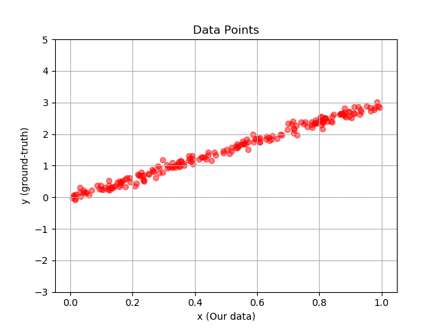

Initializing our Weights

Now, we will generate our weights $w_0$ and $w_1$ randomly.

Remember that $w_1$ and $w_0$ are supposed to be learned and they are going to be the best slope and intercept values for our line, after the training is done!

# We are using a uniform distribution to initialise our random weights
w_1 = np.random.uniform(-2,-3,1)
w_0 = np.random.uniform(0,2,1)

Now, these are some random values for the line that we want to learn. Namely, here is the equation of the initial line, before training and fine-tuning its slope, $w_1$ , and intercept, $w_0$ :

$y_{hat} = w_1 \times x_1 + w_0 \times x_0$ Since $x_0 = 1$ : $y_{hat} = w_1 \times x_1 + w_0$

This random line can be visualized using these weights as its slope and intercept and of course by plugging in our data, $x_1$ . Let’s see our does this line fit our data:

# We are generating some random weights
w_1 = np.random.uniform(-2,-3,1)
w_0 = np.random.uniform(0,2,1)
x_0 = 1
# The line
y_hat = w_1*x_1 + w_0*x_0
plt.scatter(x_1, y, s=area, c='r', alpha=0.5)
# We can also show the error
plt.plot(x_1, y_hat, '-b', label = "SSE= %.2f" %SSE(y, y_hat))
plt.grid()
plt.title('Initial Line')
plt.xlabel('x')
plt.ylabel('y')
plt.legend()
plt.ylim(-3,5)
plt.show()

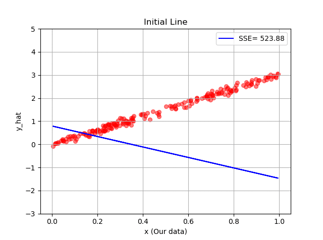
Note that I have purposely initialised our line so terribly, to show you how even such a terrible initial line with such terrible slope and intercept, can be trained by the power of machine learning and neural networks.

Training our Neural Network

Now, as always we will decide on a number for our training cycle, that is our epoch (i.e., epoch=300). We will need a small enough learning rate, $\eta = 0.001$ . Through our forward pass, we take all out 200 examples, $x_1$ , and pass it through our neural network, namely, we compute out $Z$ , $y_{hat}$ , and compute our error $E$ .

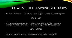
During the backpropagation, we compute the gradients of our error function, $E$ , w.r.t our weights, and update the weights. We have seen the derivations of the gradients above, and just as a reminder, the update rules for our weights are: $w_1 = w_1 - \eta\times \frac{dE}{dw_1}$ $w_0 = w_0 - \eta\times \frac{dE}{dw_0}$ Enjoy the code now:

# Number of epochs
epoch = 300
# Learning rate
eta = 0.001
# This list will save the error as training keeps going
E = []
for ep in range(epoch):
    ##################################################### Forward pass starts #################################
    Z = w_1 * x_1 + w_0*x_0
    y_hat = Linear(Z)
    error = SSE(y, y_hat)
    E.append(error) # We save the error per epoch
    ##################################################### Back propagation starts #############################
    # Here we call our functions for computing the derivatives
    dEdw_1 = dEdW_1(y, y_hat, x_1)
    dEdw_0 = dEdW_0(y, y_hat)
    # We update our parameters (i.e., the weights)
    w_1 = w_1 - eta*dEdw_1
    w_0 = w_0 - eta*dEdw_0
    # Simply every 20 epochs plot the line using the updated weights
    if ep % 20 == 0:
        # First plot our data
        plt.scatter(x_1, y, s=area, c='r', alpha=0.5)
        # Now plot the improved line
        plt.plot(x_1, y_hat, '-b', label="SSE= %.2f" %error + '\n' + "Epoch Number= %d" %(ep))
        plt.title('Initial Line')
        plt.xlabel('x (Our Data)')
        plt.ylabel('y_hat (Network Outputs)')
        plt.legend()
        plt.ylim(-3, 5)
        plt.grid()
        plt.show()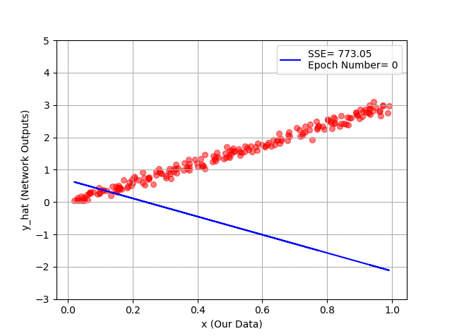

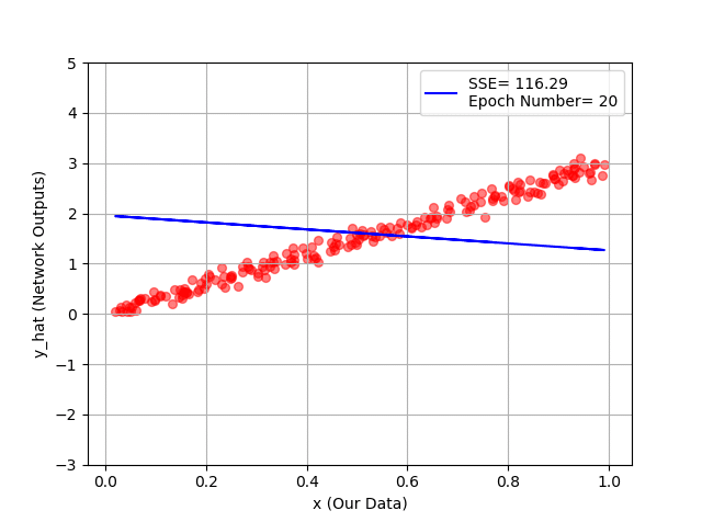
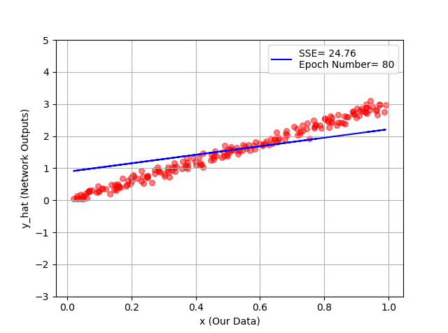
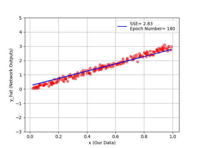
You can see hour every 20 epochs, we have a better line, and as a conclusion, a better fit to our training data!

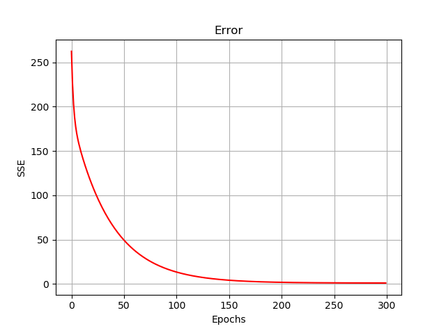
And the error function (i.e., sum squared error) is plotted down below, during our training. Below is the code for this visualisation:

plt.plot(E, 'r')
plt.grid()
plt.title("Error")
plt.xlabel("Epochs")
plt.ylabel("SSE")
plt.show()

The Entire Code in One Place

Below, you can see the whole code:

import numpy as np
import matplotlib.pyplot as plt
def SSE(y, y_hat):
   return 0.50*np.sum((y - y_hat)**2)
def Linear(Z):
   return Z
def dEdW_1 (y, y_hat,x_1):
   return np.sum(-(y - y_hat) * x_1)
def dEdW_0 (y, y_hat):
   return np.sum(-(y - y_hat))
N = 200
slope = 3
mu, sigma = 0, 0.1 # mean and standard deviation
intercept = np.random.normal(mu, sigma, N)
x_1 = np.random.rand(N)
y = slope*x_1 + intercept
area = np.pi*10
w_1 = np.random.uniform(-2,-3,1)
w_0 = np.random.uniform(0,2,1)
x_0 = 1
y_hat = w_1*x_1 + w_0*x_0
epoch = 300
eta = 0.001
E = []
for ep in range(epoch):
    Z = w_1 * x_1 + w_0*x_0
    y_hat = Linear(Z)
    error = SSE(y, y_hat)
    E.append(error)
    dEdw_1 = dEdW_1(y, y_hat, x_1)
    dEdw_0 = dEdW_0(y, y_hat)
    w_1 = w_1 - eta*dEdw_1
    w_0 = w_0 - eta*dEdw_0
    if ep % 20 == 0:
       plt.scatter(x_1, y, s=area, c='r', alpha=0.5)
       plt.plot(x_1, y_hat, '-b', label="SSE= %.2f" %error + '\n' + "Epoch Number= %d" %(ep))
       plt.xlabel('x (Our Data)')
       plt.ylabel('y_hat (Network Outputs)')
       plt.legend()
       plt.ylim(-3, 5)
       plt.grid()
       plt.show()
plt.plot(E, 'r')
plt.grid()
plt.title("Error")
plt.xlabel("Epochs")
plt.ylabel("SSE")
plt.show()

I do hope that you have enjoyed this post,

On behalf of MLDawn, take care 😉

Author: Mehran

Dr. Mehran H. Bazargani is a researcher and educator specialising in machine learning and computational neuroscience. He earned his Ph.D. from University College Dublin, where his research centered on semi-supervised anomaly detection through the application of One-Class Radial Basis Function (RBF) Networks. His academic foundation was laid with a Bachelor of Science degree in Information Technology, followed by a Master of Science in Computer Engineering from Eastern Mediterranean University, where he focused on molecular communication facilitated by relay nodes in nano wireless sensor networks. Dr. Bazargani’s research interests are situated at the intersection of artificial intelligence and neuroscience, with an emphasis on developing brain-inspired artificial neural networks grounded in the Free Energy Principle. His work aims to model human cognition, including perception, decision-making, and planning, by integrating advanced concepts such as predictive coding and active inference. As a NeuroInsight Marie Skłodowska-Curie Fellow, Dr. Bazargani is currently investigating the mechanisms underlying hallucinations, conceptualising them as instances of false inference about the environment. His research seeks to address this phenomenon in neuropsychiatric disorders by employing brain-inspired AI models, notably predictive coding (PC) networks, to simulate hallucinatory experiences in human perception.

Add a comment

By using form u agree with the message sorage, you can contact us directly now