Deriving the Gradient Descent Rule (PART-2)

Home

/

Deriving the Gradient Descent Rule (PART-2)

What Will You Learn?

In our previous post, we have talked about the meaning of gradient descent and how it can help us update the parameters of our Artificial Neural Network (ANN). In this post we will actually mathematically derive the update rule using the concept of gradient descent. We will also look at a NUMERICAL example and literally update the weights of a neural network by hand, to make sure we understand the concept. So, by the end of this post, you will have a good understanding of how to derive the update rule for the parameters of your network, given an error function of choice, using the concept of gradient descent that we have discussed in our previous post. I am ready when you are 😉

Let's derive the Update Rule

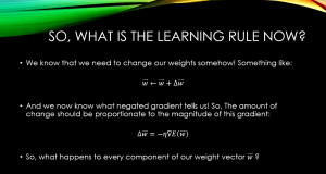
As you remember, we said that the update rule for a given weight, $w_i$ , (generally speaking) is:

$w_i \leftarrow w_i+\Delta w_i$

where:

$\Delta w_i=-\eta \frac{\partial E}{\partial w_i}$

And we emphasized that $\frac{\partial E}{\partial w_i}$ is called the gradient of our error, $E$ , with respect to our parameter, $w_i$ . Finally, we talked about $\eta$ which is our learning rate (a.k.a., the step size). Now it is time to consider a quite simple neural network, with some weights to be learned, and an error function of choice to be minimized. Consider the simple neural network below:

Figure 1: A Simple Neural Network

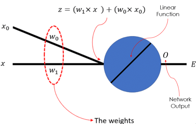
In this network, we have a 1-dimensional input data, $x$ , with a bias unit, $x_0$ , that is always equal 1, by definition. We have 2 sets of weights $w_0$ and $w_1$ , which we are trying to learn using gradient descent. The actual big blue circle is a linear neuron and $O$ represents the output of the neural network. As you can see, the input data and the weights are linearly combined to make $z$ , which is also called the pre-activation of the neuron. We will further define an error function, $E$ , that we are trying to minimize by learning an appropriate set of values for our weights. Let’s define an error function:

$E(\vec w)= \frac{1}{2} \sum_{d \in D}^{} (t_d - o_d)^{2}$

You notice that this error is a function of the weight vector, which is a vector of all the weights in our neural network to be learned. So, for every input training data $d$ , in our training set $D$ , we generate the output of our model, that is $o_d$ . Then we compute the squared difference between this output and the desired output $t_d$ . We compute this squared difference for every input data, and sum them all up and finally divide it by 2, to compute the total error across the entire training set. So, you can see that minimizing this error across the entire training set, means that for every input data $d$ , the output of our model $o_d$ is getting quite close to the target value $t_d$ , which our ground-truth.

One a side note, there is a very good reason why we have the square operation and the division by 2, in this definition of error. I have explained this in details in my course “The Birth of Error Functions in Neural Networks”. Click here to enroll (It is Free!)

So, now we need to take the derivative of our error function with respect to every one of the weights in our network. This will be the gradient of the error with respect to the weights. As a result, for every weight $w_i$ in our network, the derivative of the error $E$ with respect to that weight, which is denoted as $\frac{\partial E}{\partial w_i}$ , is computed as follows:

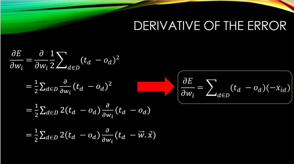
Figure 2: Deriving the Derivative of the Error w.r.t the Weights

Please note that $x_{id}$ , means the $i^{th}$ dimension of the $d^{th}$ training example.

In other words, if a weight connected to the $i^{th}$ dimension of the input, $w_i$ , then that weight can only be effected by that dimension of the input, and NOT the other dimensions! This is why when computing the gradient w.r.t $w_i$ we are only considering the $i^{th}$ dimension of the input $x$ , in the derivations above.

Now we have the gradient and it is time to incorporate that in $\Delta w_i = -\eta \frac{\partial E}{\partial w_i}$ , to measure the amount by which we need to change every weight $w_i$ :

Figure 3: Deriving the Actual Change to be Applied to the Weights

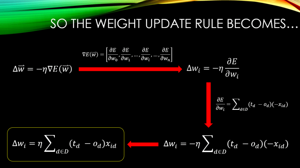
So, what this means is that by initializing our weights randomly, we will keep them fixed and pass the entire training set through our neural network and generate the outputs for each of the training examples. Then we will compute the error across all of these outputs using our error function and ground-truth labels. For a given learning rate, $\eta$ , the computed $\Delta w_i$ tells us how much we need to change, $w_i$ , in order to minimize the total error, $E$ , the fastest, as discussed in our previous post on Gradient Descent. Finally, we will add this to the current value of our weight in order to update that weight, using the learning rule:

$w_i \leftarrow w_i+\Delta w_i$

A Numerical Example for the Whole Process

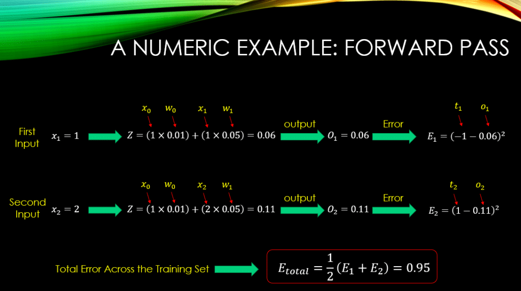
I am a big fan of simplicity, so let’s give a super simple example. We will define a training set of 2 training data (I know, too small but it is easier to understand). The neural network is the same that is depicted in Fig.1. In this neural network, please note that $x_0$ is called the bias unit and it is always equal to 1, that is to say $x_0=1$ . As a result the only input from which we will be able to feed in our training data into the neural network would be through $x$ . This means that our training data are 1-dimensional. Moreover, we will have to initialize our 2 weights randomly as well and define a learning rate. Finally, in our training set, for every training data, we will also have a ground-truth, so that we could actually compute the error and update the weights in the network. So, all of these are defined as follows:

Training Data: $x_1$ =1 and $x_2$ =2
The Ground Truth: $t_1$ =-1 and $t_2$ =1
The weights of the neural network are initialized randomly: $w_0$ =0.01 and $w_1$ =0.05
Finally let’s set the learning rate: $\eta$ =0.01

Now we will input every data point into the network according to Fig.1, compute the outputs $O$ , and compute the error for each of the outputs. This is called the forward-pass phase where the data travels from the input’s side to the output’s side of a neural network.

In all of the following derivations, $x_i$ is the $i^{th}$ training example. And as always, $x_0$ is the bias unit that is always equal to 1! Finally, $o_i$ , $t_i$ , and $E_i$ , represent the output, ground-truth, and error value for the $i^{th}$ input training data.

Figure 4: The forward-pass for Computing the Total Error Across the Training Set

So, we have computed the individual errors, summed them, and divided them by 2, and computed the total error. Now for each of the 2 weights in our network, we will have to compute the gradient of the error according to our derivative rule that we have derived, and then we will multiply the gradient by the learning rate to learn the amount we will have to change the current value of our weights. This is called the Backward phase where we back-propagate the gradients from the output side towards the input side of the network, in order to learn the degree by which we will have to increase/decrease every single weight in our neural network.

Finally we will add this value to the old value of our weights, to compute their new values. This is called LEARNING! We are learning the weights based on the errors that we make for every training data! Now, let’s update $w_0$ :

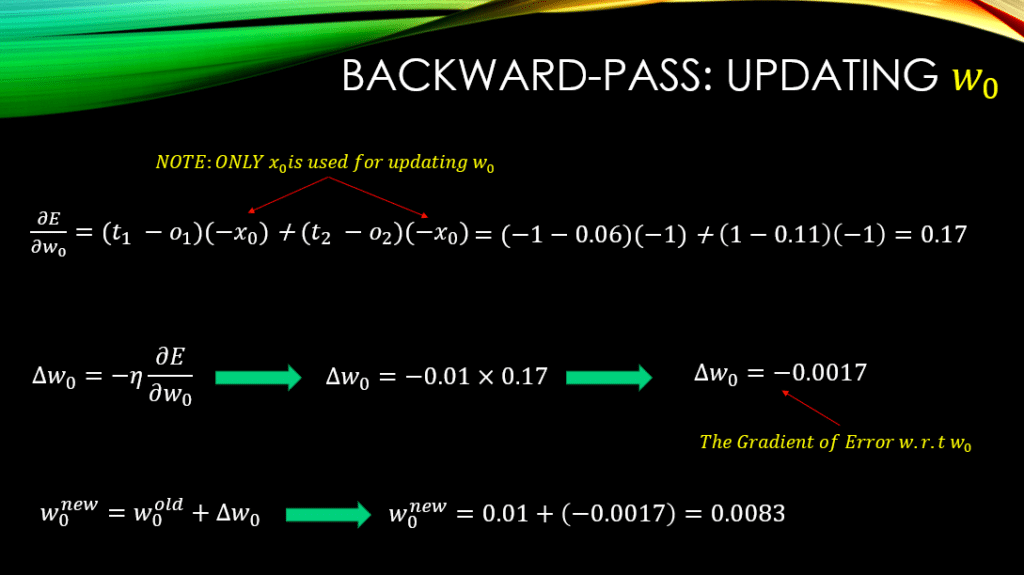
Figure 5: The Backward-Pass where we Compute the Gradient of the Error with respect to $w_0$ in order to Learn it

You note that the only inputs that we have used for computing the gradients in here, is the bias unit and NONE of the training examples in our training set. Why? Because that is the ONLY input that is connected to $w_0$ and the actual training data that are being inputted to the neural network are connected to $w_1$ and NOT $w_0$ ! So, now we have a new value for our $w_0$ ! Now, let’s update $w_1$ :

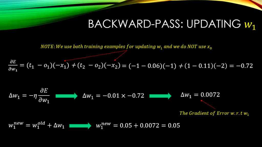
Figure 6: The Backward-Pass where we Compute the Gradient of the Error with respect to $w_1$ in order to Learn it

You see that we are using all of our training examples to learn $w_1$ ! And we are NOT using the bias unit $x_0$ as it is NOT connected to $w_1$ ! So, now we have a new value for our $w_1$ .

Conclusions

Gradient descent is quite an interesting approach but it surely has some issues and there are ways to alleviate those issues. In the next post, we will look at a variation of gradient descent, called, the stochastic gradient descent that strives to address the issues in the traditional gradient descent.

Until then on behalf of MLDawn,

Mind yourselves 😉

Author: Mehran

Dr. Mehran H. Bazargani is a researcher and educator specialising in machine learning and computational neuroscience. He earned his Ph.D. from University College Dublin, where his research centered on semi-supervised anomaly detection through the application of One-Class Radial Basis Function (RBF) Networks. His academic foundation was laid with a Bachelor of Science degree in Information Technology, followed by a Master of Science in Computer Engineering from Eastern Mediterranean University, where he focused on molecular communication facilitated by relay nodes in nano wireless sensor networks. Dr. Bazargani’s research interests are situated at the intersection of artificial intelligence and neuroscience, with an emphasis on developing brain-inspired artificial neural networks grounded in the Free Energy Principle. His work aims to model human cognition, including perception, decision-making, and planning, by integrating advanced concepts such as predictive coding and active inference. As a NeuroInsight Marie Skłodowska-Curie Fellow, Dr. Bazargani is currently investigating the mechanisms underlying hallucinations, conceptualising them as instances of false inference about the environment. His research seeks to address this phenomenon in neuropsychiatric disorders by employing brain-inspired AI models, notably predictive coding (PC) networks, to simulate hallucinatory experiences in human perception.

Add a comment

By using form u agree with the message sorage, you can contact us directly now