

When training a model, we strive to minimize a certain error function (). This error function gives us an indication as to how well is our model doing on our training data. So, in general, the lower it is, the better our model is doing on the training set.
Make no mistake! We almost never want to keep training our model until the error is 0, or too small! Most likely, this would mean that the model has over-fitted (i.e., memorized) the training data. Thus, it will have a high generalization error when confronted with the unseen test data! So, we should be looking for a good local minima, and not a global minima!
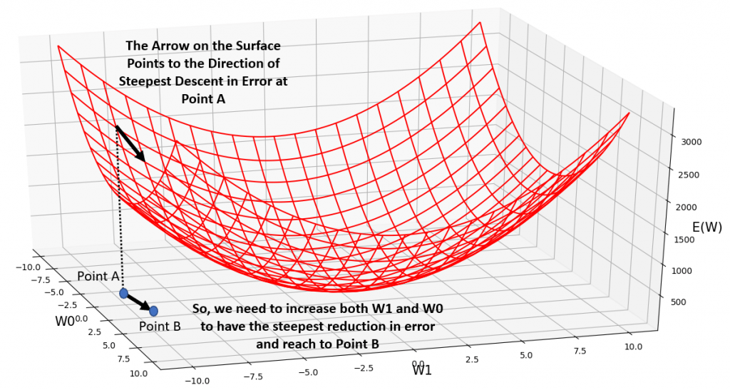
So, for example in the case of training a neural network, we keep increasing and decreasing the weights inside our neural network, and search on the error surface. The question is:
How should we increase/decrease our weights (there could be millions of such weights in our neural network), to lower our training error (E) as much as possible!
So for example, consider the simple neural network down below, which has just 1 linear neuron, and 2 learnable weights:
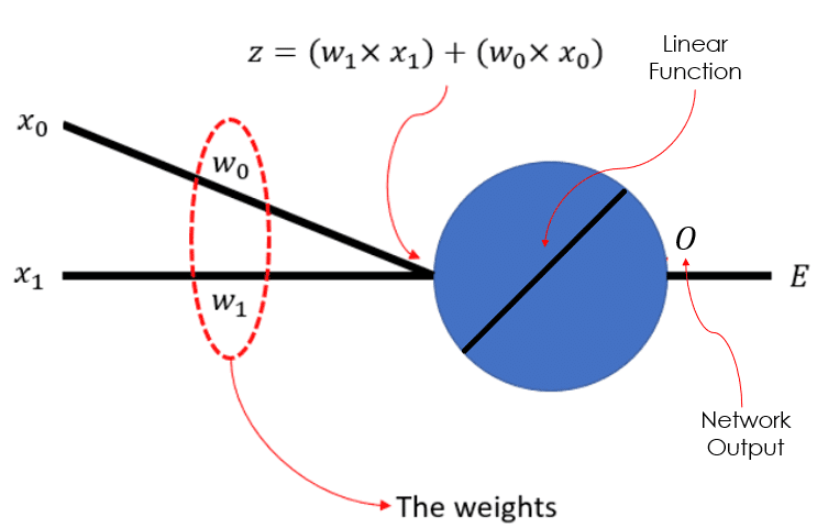
So, the question is how should we change the weights, and
, so that our error,
, would become suitably small. In other words:
Given a set of input data (say training data), some randomly chosen values for our weights, we can compute the resultant error using our error function (Means Square Error, Cross-Entropy, etc.). So how should we change our weights at every step to have the steepest descent in the value of our error (i.e., learning the patterns in the training data).
By taking the partial derivative of our error, , w.r.t each and every weight in our neural network, we can find the direction of the steepest ascent along the error surface. So, if we have
number of weights, by taking the derivative of
, w.r.t each one of them, we will get the gradient vector which has
elements as well.
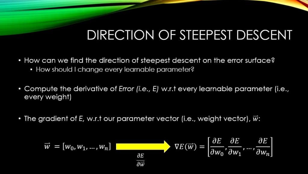
Let’s take a moment and understand what is happening here. Let’s consider the first element of the derivative vector, . It has a sign and it has a magnitude!
Let’s look at the magnitude first:
The magnitude of
shows the proportion of change in
over
, if we increase the current value of
What about the sign of this gradient?
If
, then it means that if we keep all the other weights constant, we will have to increase
, then it means that if we keep all the other weights constant, we will have to decrease
So, if we know the direction and magnitude of change for every weight (i.e., increasing or decreasing them), using the gradient, we have moved towards the direction of the steepest ascent on the error surface, as far as (pay attention!!!) ALL OF OUR WEIGHTS, are concerned!
So what is the direction of steepest descent then? Of course, the negated direction of the gradient. So, the polar opposite of that!
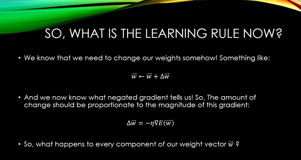
It is now clear that, both the direction of change for every weight in our neural network, and the magnitude of that change, have some connection with the gradient of our error, , w.r.t to every one of those weights. As a result, for a given weight parameter,
, we will compute an amount of change,
(which is tightly tied with our gradient
), and add it to our current value for
.
We mentioned that we need to negate
in order to move along the steepest descent on the error surface (rather than steepest ascent). So that is all about the direction of movement. Regarding the magnitude of movement, we know that the magnitude of
. We tend to multiply
(pronounced ‘eta’), also known as the learning rate!
So we negate the value of the gradient, and then multiply the result by our learning rate, to see how much we should change our wights. This is all nicely summarized down below:

Author: Mehran
Dr. Mehran H. Bazargani is a researcher and educator specialising in machine learning and computational neuroscience. He earned his Ph.D. from University College Dublin, where his research centered on semi-supervised anomaly detection through the application of One-Class Radial Basis Function (RBF) Networks. His academic foundation was laid with a Bachelor of Science degree in Information Technology, followed by a Master of Science in Computer Engineering from Eastern Mediterranean University, where he focused on molecular communication facilitated by relay nodes in nano wireless sensor networks. Dr. Bazargani’s research interests are situated at the intersection of artificial intelligence and neuroscience, with an emphasis on developing brain-inspired artificial neural networks grounded in the Free Energy Principle. His work aims to model human cognition, including perception, decision-making, and planning, by integrating advanced concepts such as predictive coding and active inference. As a NeuroInsight Marie Skłodowska-Curie Fellow, Dr. Bazargani is currently investigating the mechanisms underlying hallucinations, conceptualising them as instances of false inference about the environment. His research seeks to address this phenomenon in neuropsychiatric disorders by employing brain-inspired AI models, notably predictive coding (PC) networks, to simulate hallucinatory experiences in human perception.


Responses
[…] our previous post, we have talked about the meaning of gradient descent and how it can help us update the parameters […]