What is the Delta Rule? (Part-2)

What We Have Learned So Far ...

So far, we have learned that the Delta rule guarantees to converge to a model that fits our data the best! It just so happens that the best fit might be a terrible model but still it is the best that the Delta rule has been able to come up with. We also learned that the Delta rule uses Gradient Descent as the optimization tool, to search the hypothesis space of possible weights for our Artificial Neural Network (ANN). All of these ideas are available in out previous post.

What We Will Learn Today ...

We have been talking about the hypothesis space and the gradient descent algorithm used by the Delta rule to search this hypothesis space of weights for the neural network. However, we have never actually had a glimpse into this hypothesis space. In this post, we will consider a simple neural network and actually visualize the entire hypothesis space of weights with their corresponding error values. This will help you understand, what it really means to say that:

We would want to find the best fit model, by finding the weights that would minimize the error on our training data!

Building a Neural Network

Let’s consider the following simple neural network down below. Every input training data is 2-dimensional, denoted by x0 and x1. We have a weight value to be learned for each dimension, w0 and w1. The weights and input values are linearly combined to constitute Z. Then Z, that holds the pre-activation value for our linear neuron (in blue), will go through a linear transformation through the neuron to produce the output O. Then the error will be computed and then using Gradient Descent we will search for the weights (i.e., by modifying the current weights) that would minimize this error over the entire training set.

Fig.1: A simple neural network for 2-dimensional data with a linear unit. 

The error function that we are going to be using is the simple yet quite popular Sum Squared Error (SSE) function, described below:

Fig.2: The Sum Squared Error (SSE) function that we will be using for our simple neural network depicted in Fig.1

Note that the error is obviously a function of the input training data as well, and not just the weights! However, we tend to consider the weights in our mathematical representation of the error function, as these weights are the ones that we could alter and tune to minimize the error, while we don’t have the same control over our training data. Note that in Fig.2, D is our entire training data, and the error could be explained as the following, in a more intuitive fashion:

For any given set of weights, the SSE error function measures the sum of squares of difference of the output of the model and the ground truth, across the entire training set D. The whole thing is divided by 2, for mathematical convenience (I will tell you why in later posts)

How Could Gradient Descent Help Find the Minimum?

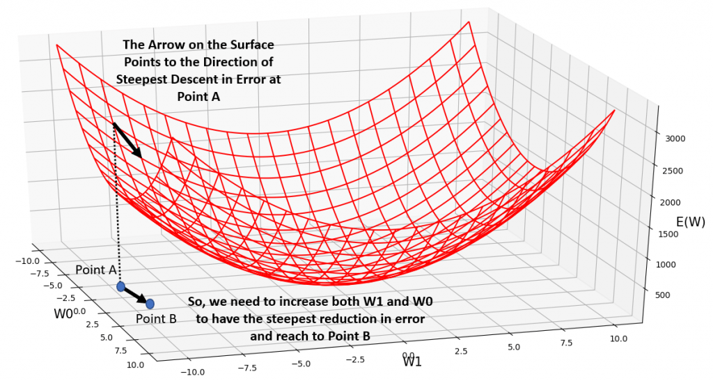
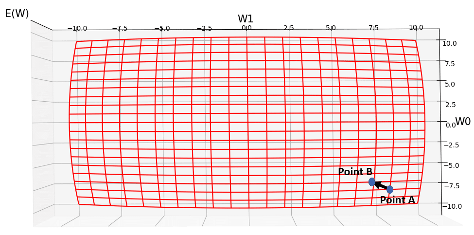
In Fig.3 below, you can see the plooted surface of our SSE error function for a synthetic dataset, across a wide range of possible weight values for our simple neural network, depicted in Fig.1. You can see that it clearly has a global minimum, and that minimum my friends, happens at a specific value for w0 and a specific value for w1. Any other value for w0 and w1 would correspond to a higher error value on the error surface. Note that while training a neural network, we rarely have a nice behaving error surface such as this one. It tends to be wobbly with loads of local maximums and and minimums. However, this is not the topic of this post ;-). It is important, for now, to appreciate the fact that:

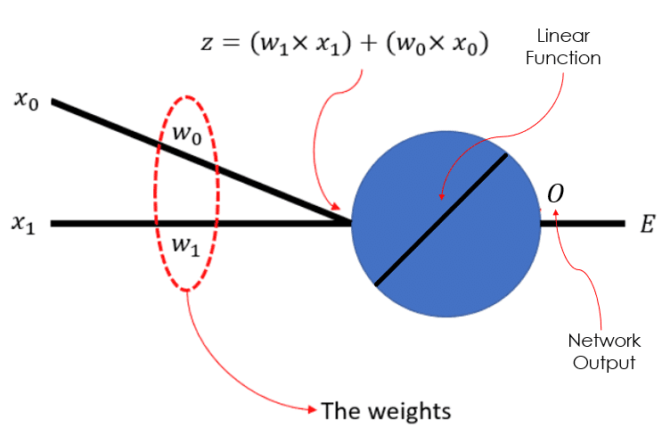
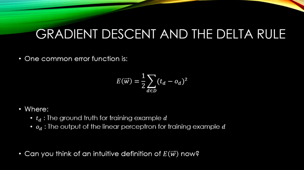
Given the way we have defined the error function, for linear units, the error surface is always a parabolic with a single global minimum.

Typically, before gradient descent would start to even explore the hypothesis space of possible weights for the neural network, we would have to initialize our weights to some random values. Let’s say we have chosen the values -5.0 and -10 for w0 and w1 respectively. Notice Point A in Fig.3, on the W0-W1 plain which corresponds to this randomly initialized set of weights. The corresponding error, on the error surface reads a value almost close to 3000 (Ignore the little arrows and other stuff for now ;-)). Here is the question:

How should I change w0 and w1, so that the error would reduce the fastest? What is the direction of this steepest descent in error?

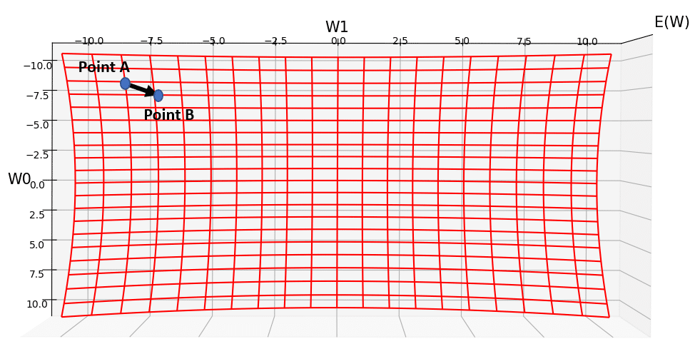
Gradient Descent, searches the hypothesis space of possible weights (i.e., the W0-W1 plain), and finds the direction of the steepest descent in your error, and tells you how much you need to change all of your weights, so that with your new set of weights, you will have had the steepest decrease in your error from the initial old value (3000). The result is moving from Point A to Point B in fig.3. So, after gradient descent took 1 step of optimization, the new set of weights at Point B would be almost 0.0 for w0 and lamost -9.0 for w1. You can see that the new value for error has dropped to nearly 2500. As gradient descent would take more and more steps of finding the direction of steepest descent on in the error surface, the parameters of the model keep updating and updating, until we reach the global minimum. You can see the same error surface from top and bottom views in Fig.4, and Fig.5, respectively.

Fig.3: Side view of the Sum Squared Error Function. See how Gradient Descent determines the direction of the steepest descent in error, starting at Point A, and determines the new values of our weights at Point B.

Fig.4: Top view of the Sum Squared Error Function. This gives you a more clear idea as to how Gradient Descent modifies our weights in the same direction of the steepest descent on the error surface.

Fig.5: Bottom view of the Sum Squared Error Function.

Conclusions

In this post, without going too much into the details of the Gradient Descent algorithm, we learned that Gradient Descent searches the hypothesis space of the parameters (i.e., the weights of the neural networks in this case), and it keeps changing the parameters in a way that we would have the steepest reduction in the error at any step of the optimization. So, in conclusion, we can say that:

Given an initial set of random weight values, Gradient Descent finds a weight vector that minimizes the error. We have to know that Gradient Descent is a repetitive search algorithm that at each step, it strives to modify the weights in the direction of the steepest descent  in error, along the error surface shown in Fig.3

I do hope that this has been informative for you,

Until next time, on behalf of MLDawn,

Take care 😉

Leave a Comment

Your email address will not be published.